Note: This is a linkpost for the Metaculus Journal. I work for Metaculus and this is part of a broader exploration of how we can compare and evaluate performance of different forecasters.
Short summary
- It is difficult to interpret the performance of a forecaster in the absence of a sensible baseline.
- This post proposes a (novel?) experimental metric that aims to help put forecaster performance into context
- From her subjective perspective, a forecaster assumes that her prediction is equal to the true probability of an event (otherwise she would have issued a different prediction). The idea is to take this assumption at face value and assume that a forecasters’ predictions correspond to true event probabilities. Based on that, we can compute an subjective expected score and compare the actual score against that
- All of this is very exploratory (and maybe slightly crazy?), but it's intellectually interesting and might potentially lead to useful insights.
Introduction
"How good is this forecaster" is a question of great interest to anyone who is trying to assess the credibility of a forecast. I recently wrote about how difficult it is to establish that there is a significant difference in performance between two forecasters. Evaluating a forecaster not only in relative, but in absolute terms is even more difficult.
Imagine, again, that you're King Odysseus of Ithaca. Times are rough. You haven't been home for twenty years, your kingdom is a mess and new dangers are looming on the horizon. You could really need some divine help or some prescient counsel. Your trusted maid Eurycleia suggested you go off to consult the oracle of Delphi.
You: "Are you sure it's worth it? How good is the oracle of Delphi really"?
Euryclia: "It's the best oracle in Greece!
You: "Even if Delphi is better than the others... they might all be terrible! And it's a really long journey!"
Euryclia: "You really don't like travelling, don't you?"
You: ...
Euryclia: "To soon? I'm sorry. Listen, I think Delphi is really good. You should go."
You: "But how good exactly!"
Euryclia: "It says on their website they have a Brier score of 0.085 on Metaculus!"
You: "But what does that even mean? maybe they only predicted on the easy questions!"
Euryclia: "The divine oracle of Delphi made a forecast on every single question on Metaculus."
You: "But maybe all questions on Metaculus are easy!"
Euryclia: looks at you sternly
You fall silent. You still think you have a point. But Euryclia will have nothing of it. Sure, officially you are the king. But you're a wise king and you know your place.
Meaningful comparisons
You lie awake in bed at night pondering the question. The problem with the Brier score, the log score, or really any other scoring rule used to evaluate predictions is that the score you get is mostly meaningless without anything sensible to compare it against.
For binary forecasts (outcome is either 0 or 1) the 'naive forecaster' is a natural, albeit not very helpful, baseline. The logic of the naive forecaster is that "surely the probability of any event must always be 50% - it either happens or it doesn't". Accordingly, the naive forecaster always assigns 50% probability to any outcome. Another possible baseline is the 'perfect forecaster' who is always correct. This, again, is not tremendously helpful.
The problem with constructing a baseline is that we can’t really say how “hard” a forecasting question is - we don’t know the “true probability” of an event [1].
You pause for a second. Maybe we could compare a forecaster against the score she herself should expect to get? Forecasters are usually evaluated using a proper score. A proper scoring rule is a metric that is impossible to cheat: you can't do any better than predicting your actual belief. From a forecaster’s perspective, if you predict 0.7 on a binary question, then you’re really expecting a 70% probability that the question will resolve yes.
Now you may be right or wrong about this, depending on whether or not your forecasts are in fact well calibrated. Calibration refers to a basic agreement between predictions and observations. One possible way to define calibration is to say that a forecaster is well calibrated if events to which she assigns a probability of x% really occur with a frequency of x%. For example, you could give a well calibrated forecaster 1 million forecasting question. Of those questions where she assigned 95% probability to "yes", 95% should really resolve "yes". Of those she assigned a probability of 7% to, only 7% should resolve "yes" etc. [2]
Regardless of whether or not a forecaster is in fact well calibrated, she is always expecting to be well calibrated when she makes her prediction (otherwise the proper scoring rule would incentivise her to make a different prediction). In her mind, the "true probability" of an event is equal to her prediction. Given a set of predictions we can therefore easily compute the score she can expect to get from her subjective perspective. If her actual score is much different from this "subjective expected score", we know something is off.
One commonly used score for binary events is the Brier score. It is computed as , where the outcome is either 0 or 1 and is a prediction that the outcome will be 1. So if the outcome is 1, your score is and if the outcome is 0, the score is . The best possible score is 0, the worst is 1, and the naive forecaster who always predicts 50% would always get a score of .
Not knowing the outcome in advance, the expected Brier score of any forecaster is.
From the subjective perspective of the forecaster the prediction should equal the true probability. The subjective expected score therefore is.
Let's call the "subjective expected score". Now, for any forecaster, you can easily compare the actual Brier score with their subjective expected score.
You lie in bed, quite excited you might have found a solution for your problem. What makes this approach so elegant is that it implicitly takes the difficulty of a question into account. If the oracle of Delphi really only forecasted on easy questions that would explain its great Brier score on Metaculus. But also she would be expected to get a low Brier score. Comparing the actual vs. the subjective expected score could be a way to know what we should expect from her and how far away she is from her own expectations! Problem solved!
Problem not solved.
Why did you, of all mortal beings, expect this to be smooth sailing?
The elephant in the room is of course that any kind of metric that compares a forecaster's score and their subjective expected score is not a proper score. The difference between the actual score and the "subjective expected score" can be cheated. For example, you could imitate the naive forecaster and always predict 50% without looking at the question. You would get an actual Brier score of 0.25 regardless of the outcome, but you would also get a "subjective expected score" of 0.25 and a perfect difference of zero.
Behaviour of the subjective expected score
Ok. But maybe there is still some merit in computing the "subjective expected score". To understand its behaviour and since you can't sleep anyway, you decide to get out your abacus and simulate some data. That's apparently the kind of man you've become in the last twenty years away from home. Your wife, Penelope, looks at you somewhat puzzled.

Behaviour for a single forecast
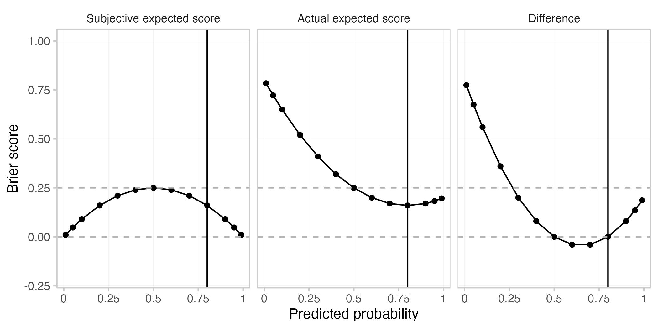
You start with the very simple case of a single forecast for a single event. This plot shows the actual expected Brier score (), the subjective expected Brier score , and the difference between the two for different predicted probabilities. The true probability of the event is assumed to be 0.8 (black vertical line).
As with every proper scoring rule, the actual expected Brier score is best (i.e. smallest) when the prediction is equal to the true probability (when ). This is not the case for the subjective expected score nor for their difference.
The following table gives an overview of the behaviour of the actual vs the subjective expected score.
| Comparison score | Interpretation |
|---|---|
| actual score < subjective expected | prediction in between 0.5 and true probability |
| actual score = subjective expected | prediction = 0.5 or |
| prediction = true probability | |
| actual score > subjective expected | prediction closer to 0 or 1 than true probability or |
| prediction on the wrong side of 0.5 |
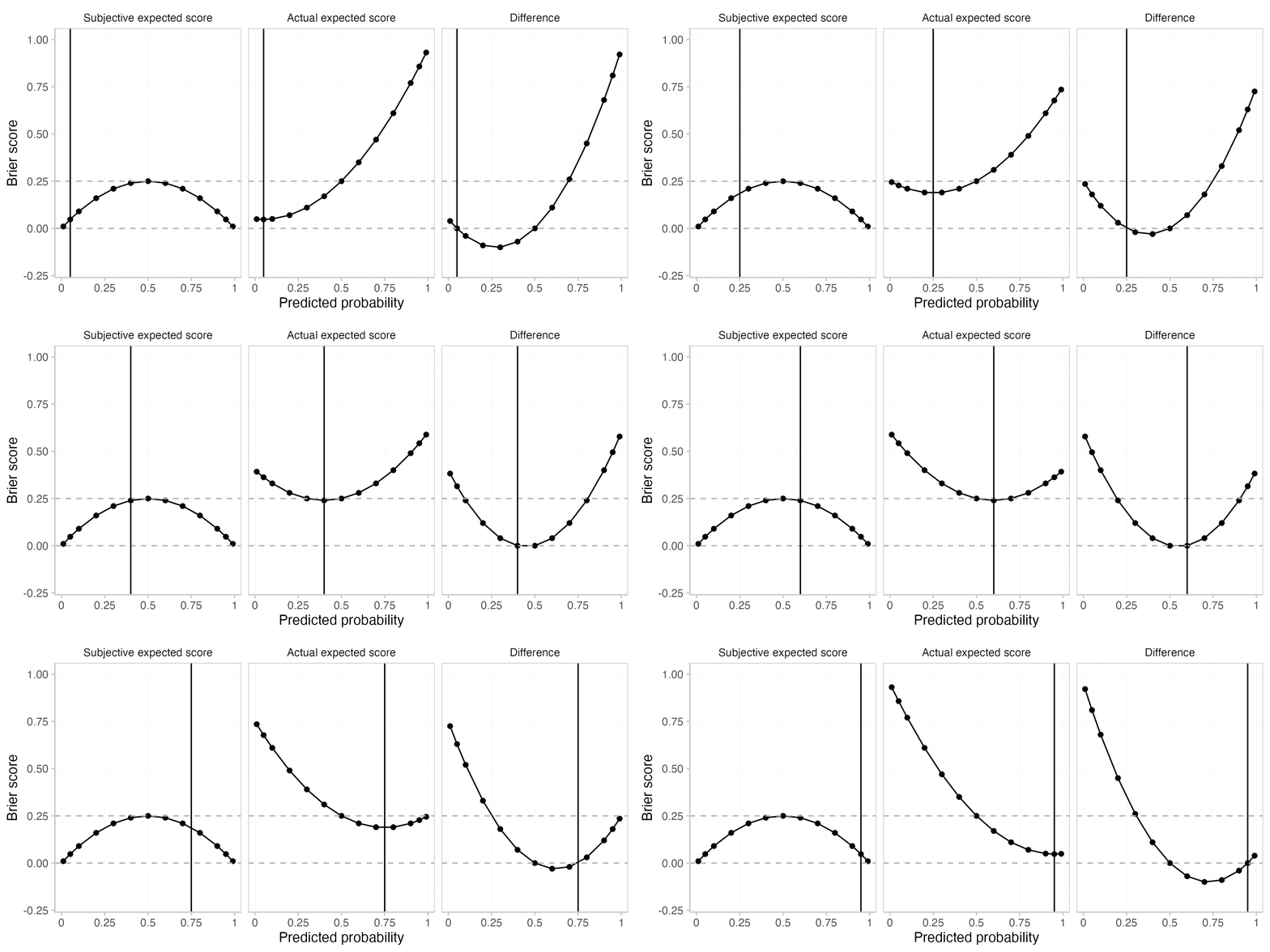
Roughly speaking, the actual expected score is greater (i.e. worse) than the the subjective expected score when the forecaster is either overconfident (making more extreme predictions than warranted) or if she is on the wrong side of maybe (predicting e.g. < 0.5 if the true probability is > 0.5 or the other way round). The actual expected score is smaller (better) than the subjective expected score if the forecaster is underconfident, but directionally correct. Both are equal if the forecaster predicts either 0.5 or if she predicts the true probability.
You're not sure it adds all that much, but since a) you really can't sleep, b) you're wife is already annoyed anyways and c) you are, after all, king Odysseus of Ithaca, you also create an animated gif that shows the above plot for different true probabilities.
Based on your observations, you form a hypothesis: Subjective expected scores and actual Brier scores are influenced by three main things:
- systematic over- and underconfidence of the forecasts
(We saw that underconfident forecasts led to subjective expected scores > actual Brier scores, and the opposite for overconfident forecasts) - undirected noise (aka "being a terrible forecaster")
(Being a terrible forecaster is widely known to be one of the top reasons why forecasters get bad scores…) - the 'difficulty' of the prediction task, i.e. whether true probabilities are close to 0.5 (hard question) or close to either 0 or 1 (easy question)
(Forecasters get better Brier scores in expectation as well as better subjective expected scores when probabilities are close to 0 or 1)
Crucially, these three factors may not have to influence both scores in the same way (note e.g. that the slopes of the curves in the above plot differ at different points). This might provide useful information.
Behaviour for a set of 1000 forecasts
You sit up straight in bed. Next, you want to analyse the behaviour across a set of multiple questions. Your wife Penelope turns around and looks at you incredulously. "Could you please stop using the abacus in bed? I can't sleep with all that clacking noise". You nod, give her a kiss, and slide out of the bed to head downstairs to your old study room. Sitting down between old and dusty parchments, you light a candle and start working on your next simulation study.
You're going to do a thousand replications of your experiment. For every replication, you simulate 1000 true probabilities observations and corresponding forecasts. True probabilities are drawn randomly from a uniform distribution between 0 and 1. The outcome was set to 1 or 0 probabilistically according to the true probabilities (i.e. the outcome is 1 with probability equal to the corresponding true probability (and 0 otherwise)). Your starting point is an ideal forecaster (predictions = true probabilities) whose forecasts you eventually modify in different ways. Lastly you compute the actual and subjective expected scores and take the mean across your 1000 simulations, leaving you with one average score for every replication.
For each of 1000 replications:
1. Draw N = 1000 true probabilities as a random uniform variable between 0 and 1
2. Create N = 1000 observations as draws from a Bernoulli distribution (drawing either a 0 or a 1) with the probability of drawing a 1 equal to the true probabilities drawn in step 1)
3. some computation (see details below)
4. Compute mean(actual Brier scores) and mean(subjective expected scores)
Over- and underconfidence
First, you're interested in what happens if you make forecasts systematically over- or underconfident. You decide to simulate increasingly over- or underconfident forecasts by converting probabilities to log odds and multiplying them with a factor smaller or greater than 1.[3]
3a. Create 5 forecasts with differing confidence bias levels 0.6, 0.85, 1, 1.15, 1.4. Values <1 represent underconfidence, values >1 represent overconfidence, 1 equals the ideal forecaster
- Convert probabilities to log odds = (log (p / 1-p))
- compute biased_log_odds = log_odds * confidence_bias
- Convert odds back to obtain probabilities with either under- or overconfidence
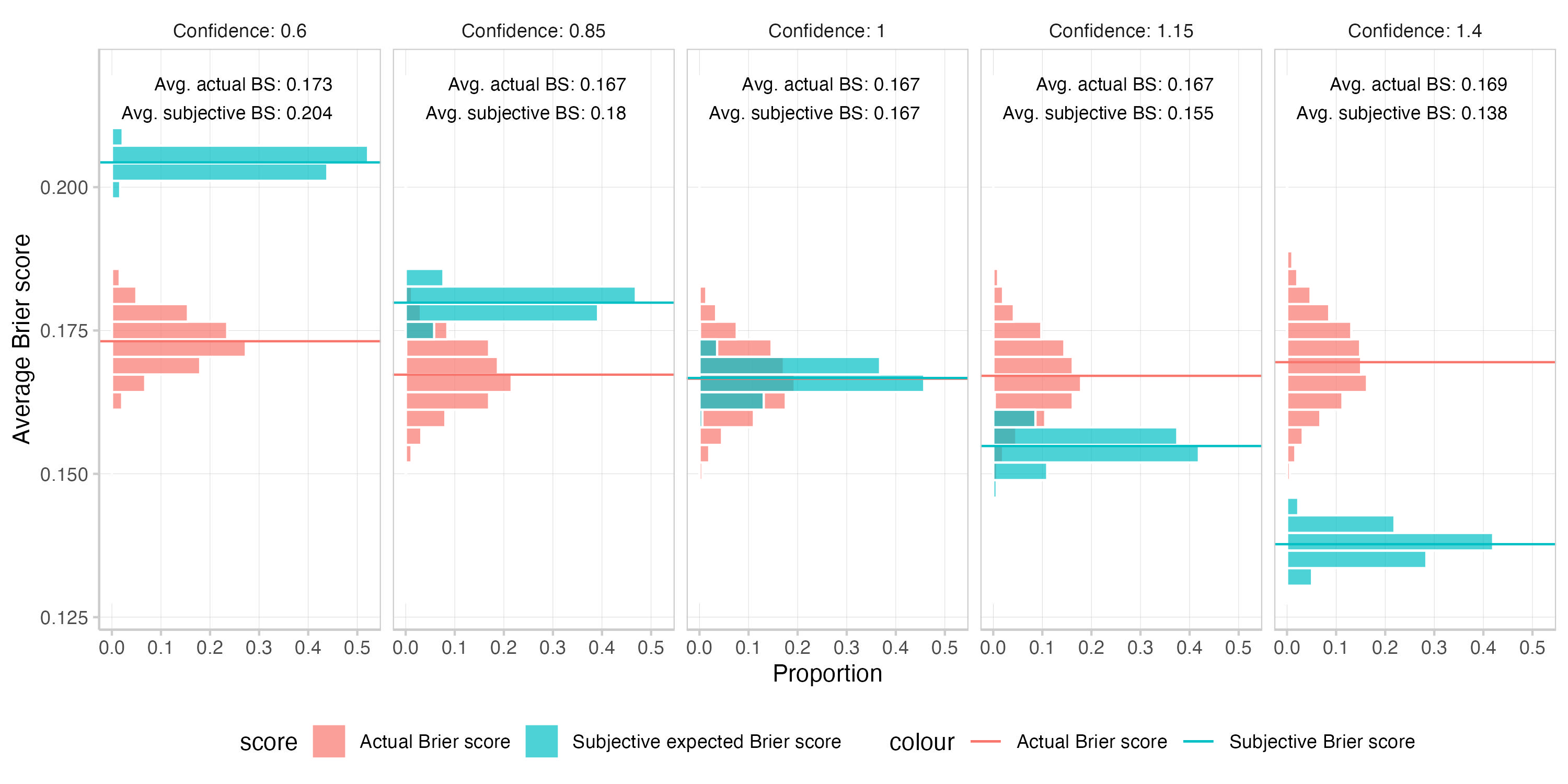
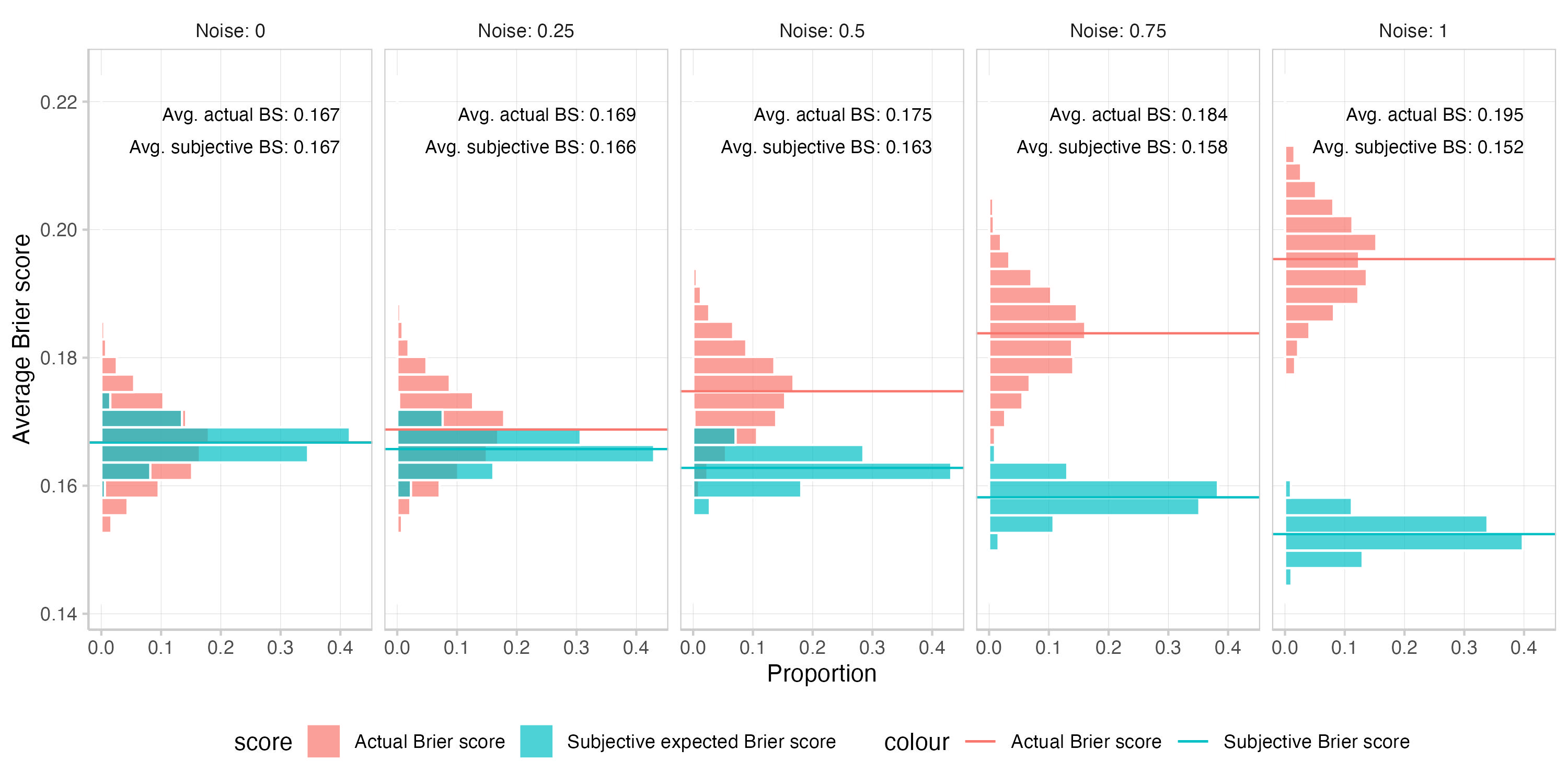
This is what you get. The first plot shows a histogram of the means of the actual and subjective expected Brier scores across 1000 replications. The second one is a calibration plot that displays predicted probabilities against observed frequencies. The third one shows a histogram of the predictions (which is essentially the information encoded in the size of the dots in the second plot).
In this particular example systematic over- or underconfidence has a much stronger influence on subjective expected scores than actual Brier scores. This makes intuitive sense, given that the expected Brier score is calculated as . When you change the prediction, you're only changing for the actual Brier score, but you're changing as well as for the subjective expected Brier score. Do that systematically in the same direction across all predictions and you end up with a strong effect.
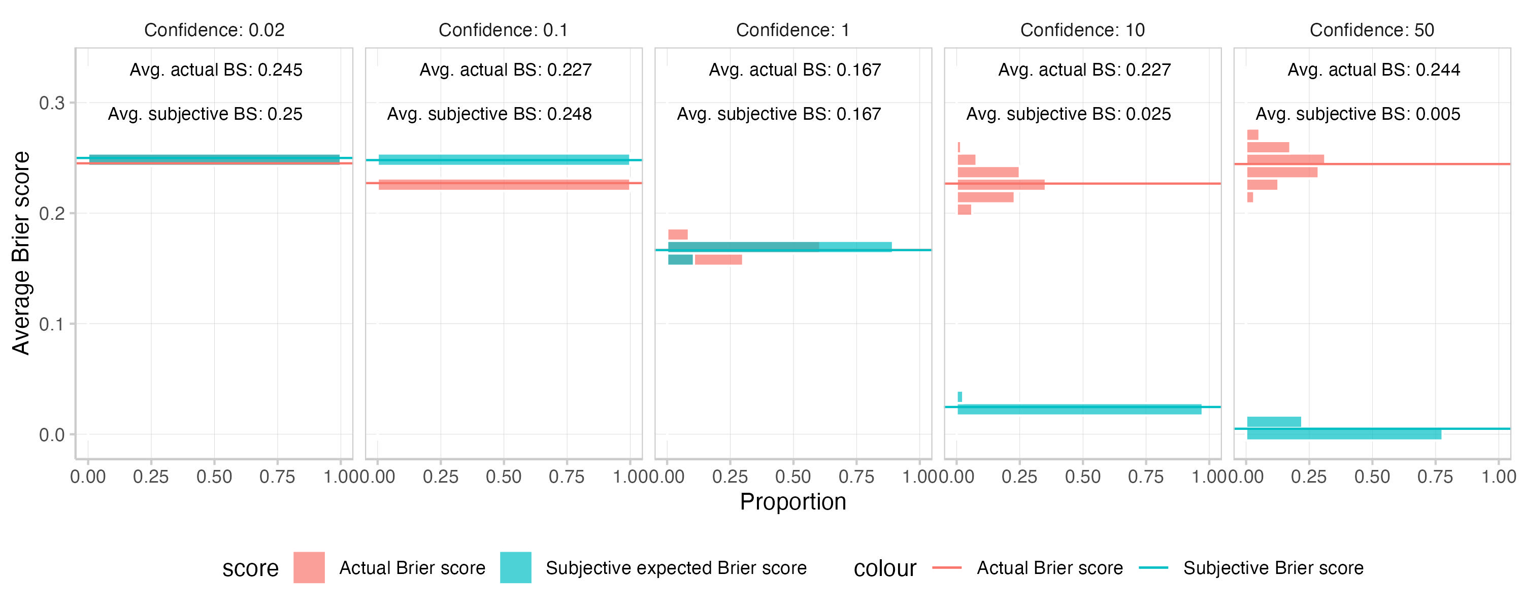
Note that if you made forecasts even more extremely underconfident than is shown in this plot (i.e. make all predictions close to 0.5), then both actual and subjective expected scores would just converge towards 0.25. This is illustrated here:
Adding noise
Next, you want to see what happens when you add random noise to the forecasts, instead of inducing systematic over- or underconfidence. Again, you operate with log odds and add random noise drawn from a normal distribution with mean 0 and standard deviation equal to the desired noise level: .
3b. Create 5 forecasts with differing noise levels, 0 (no noise), 0.1, 0.25, 0.5, 0.75, and 1
- Convert probabilities to log odds = (log (p / 1-p))
- noisy_log_odds = log_odds + N(mean = 0, sd = noise level)
- Convert back to obtain noisy probabilities
This is the result for different levels of noise:
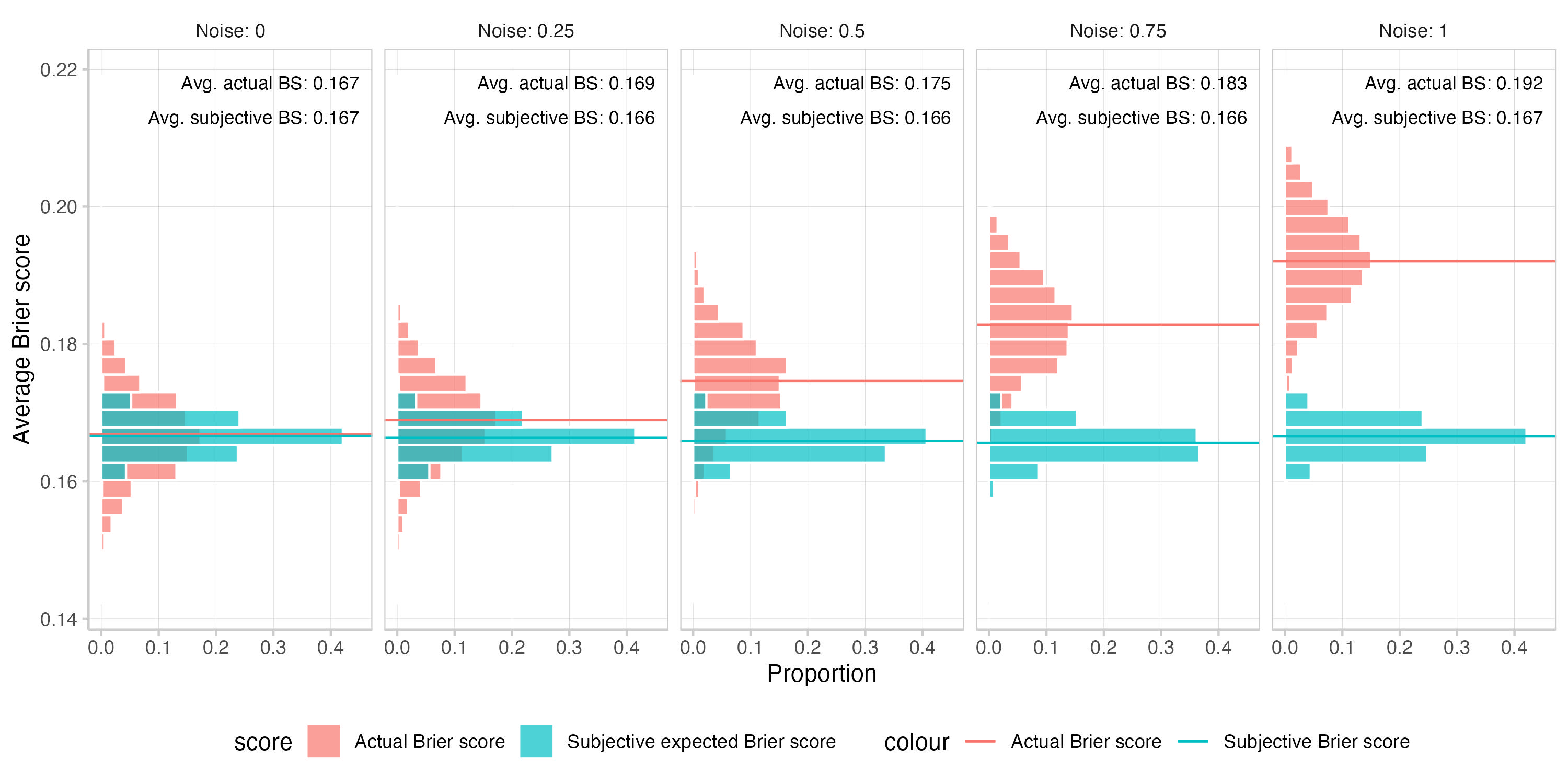
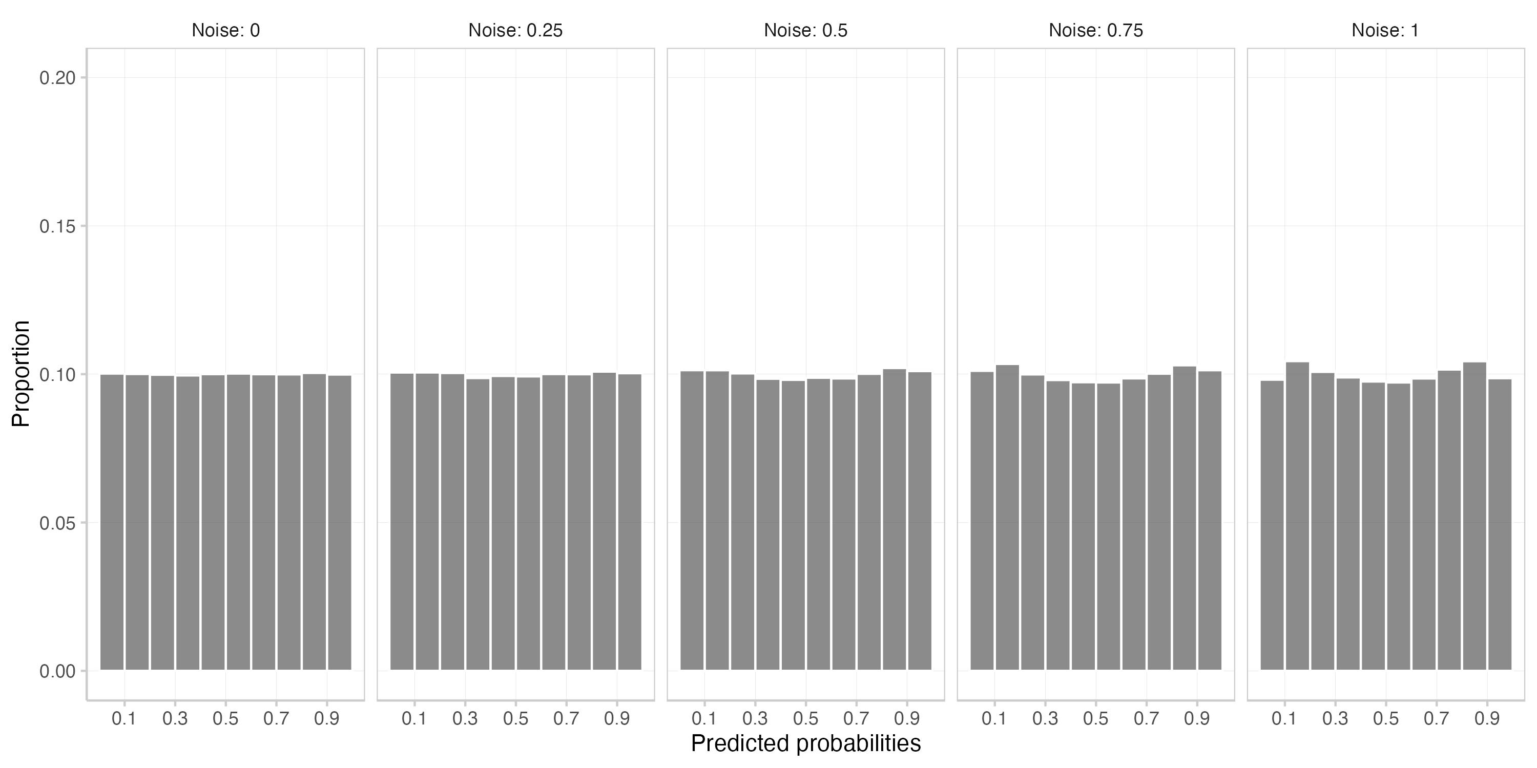
Adding noise seems to have a somewhat stronger effect on actual Brier scores than on subjective expected scores. As we can see from the calibration plots and the prediction histogram, adding noise to the log odds also introduces some overconfidence. There might be better ways to add noise than what you did - but 12th century BC abacus technology is not perfect and even your cunning has limits.
You suspect that the effect on the subjective expected scores mainly comes from the overconfidence you involuntarily introduced by adding noise on the log scale. You briefly check what would happen if you added noise on the actual probabilities, rather than on the log odds. And indeed, if you add noise to probabilities instead, the effect on the subjective expected scores vanishes almost completely. Alas, parchment is expensive and so you decide not to write your results down in detail. Instead, you just make a small note on the side (this is a trick that you learned from your old friend Fermatios).
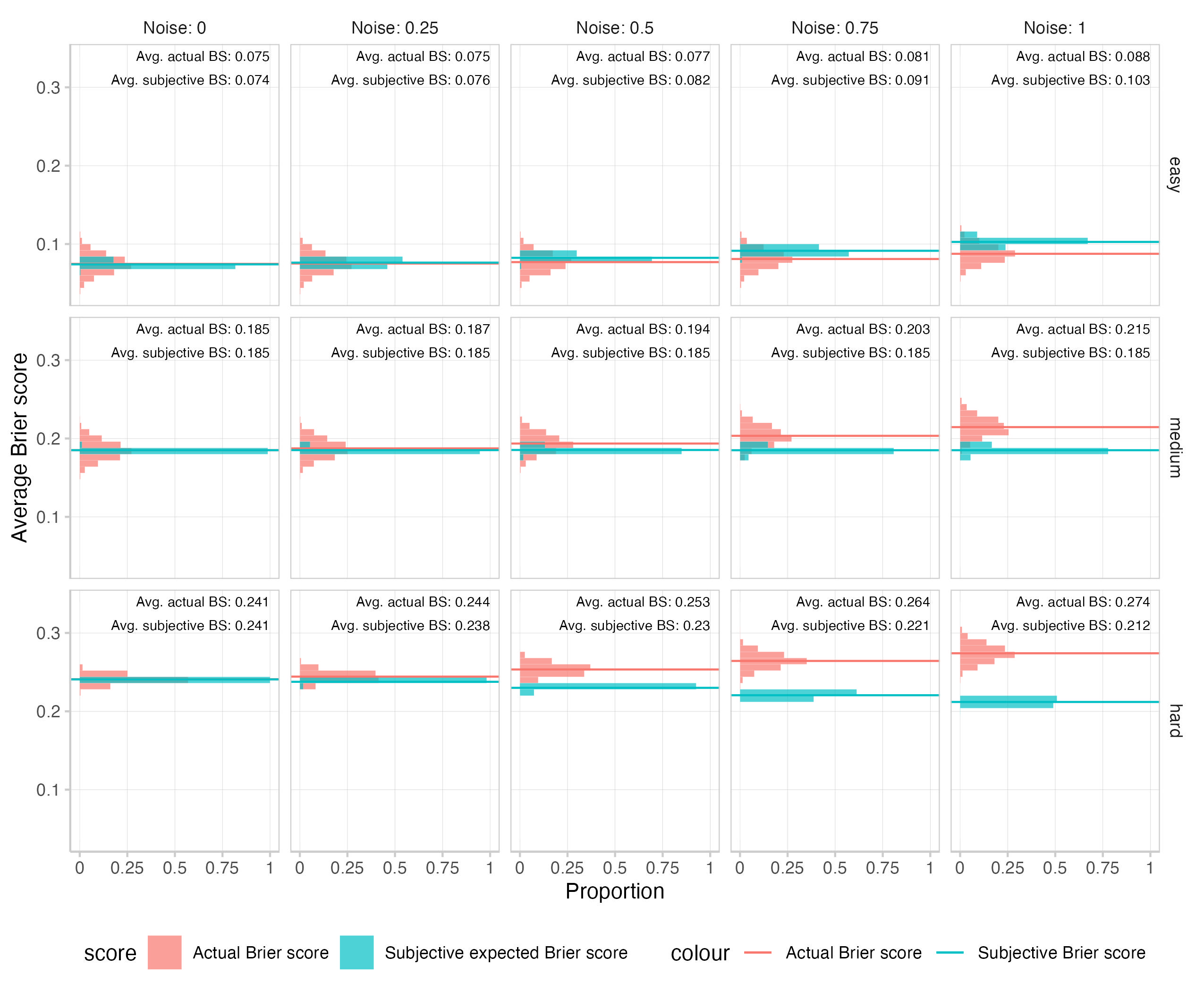
Indeed, you also check what happens if you combine noise on the log odds with underconfidence. It’s a bit of a hack, but you manage to find something of a balance between noise and underconfidence such that subjective expected scores stay more or less constant, but actual Brier scores increase. (You make another note on the side of the parchment and conclude that overall
a) noisy forecasts seem to mainly make actual Brier scores worse,
b) over- and underconfidence seem to mostly affect subjective scores, and
c) introducing noise can sometimes also mean introducing overconfidence and then you affect both, but the effect of noise on actual Brier scores is probably stronger.
Hard and easy questions
Lastly, you want to find out how question difficulty affects scores. To that end you classify questions as such:

- "easy"if or
- "medium", if or and
- "hard", if
You run your past analyses again, but this time you stratify your results by question difficulty. In reality, question difficulty is of course not observable, but you want to see what influence difficulty has on scores. Maybe that could enable you to also make inference the other way round, i.e. determine question difficulty based on observed scores.
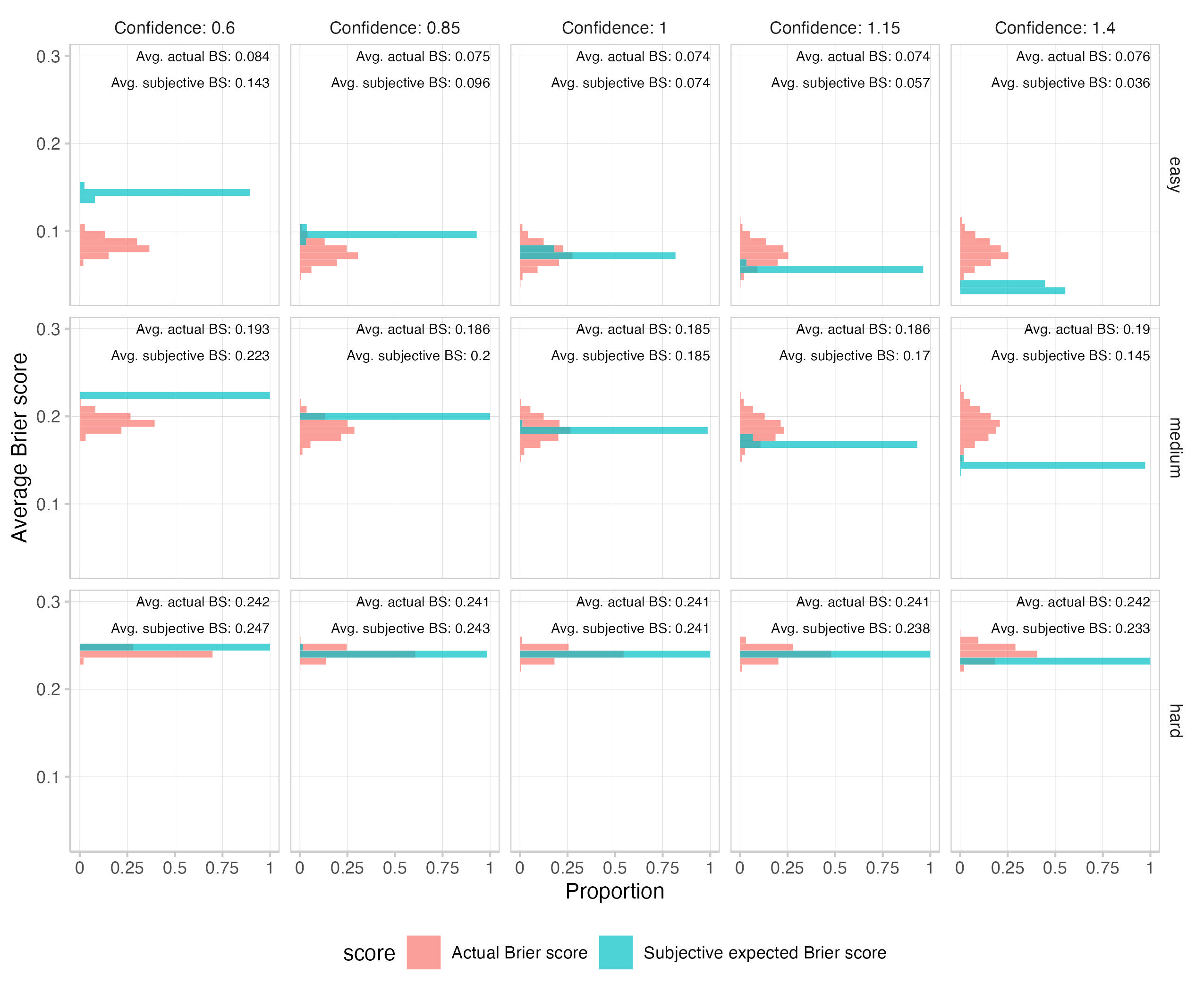
Here are the results for over- and underconfidence (0.6 and 0.85 represent underconfidence, 1 is the ideal forecaster, and 1.15 and 1.4 represent overconfidence).
We can see a clear relationship between scores and question difficulty. We also see that question difficulty mediates the influence of over- / underconfidence: Differences between actual and subjective expected Brier scores caused by over/underconfidence are largest for easy questions, and smallest for difficult questions.
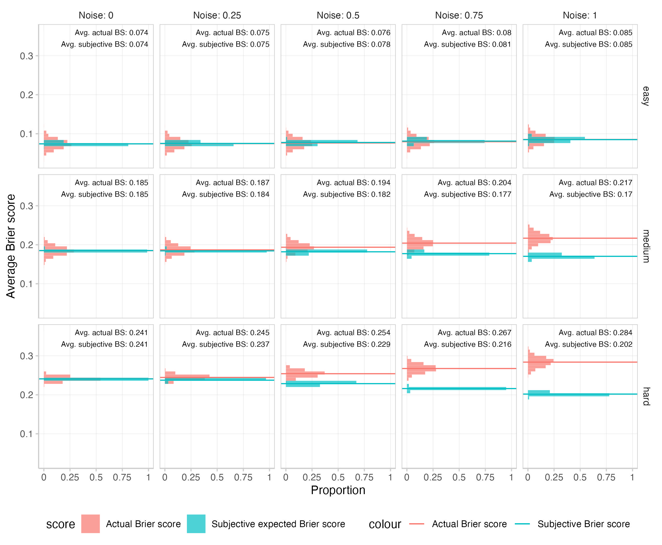
Those are the results for adding different levels of noise, stratified by question difficulty:
The pattern we can see here is a different one: Now differences between actual and subjective expected scores caused by noise tend to be largest for difficult questions, and smallest for easiest. The pattern we see here is similar for the version that combines noise and underconfidence (subjective expected scores mostly just tend to be a bit higher in particular for easy questions, see footnote[4]).
You stroke your beard and murmur to yourself "Now this is interesting". "Yes yes, very interesting indeed", you keep thinking. You sigh. Deep inside you know that you don't really have a clue of what all of that is supposed to mean.
Conclusions
Every research project needs conclusions, so you start writing. It's not that you believe your approach is completely useless - it's more that you're painfully aware that things remain complicated.
After having stared at your plots for several hours, this is your best guess of what all of this actually means (note that all of this is a matter of degrees, which the following table doesn't capture appropriately):
| low expected score | high expected score | |
|---|---|---|
| low actual score | 1) questions are “easy” and forecaster is great 2) questions are easy and forecaster is somewhat terrible, but still well calibrated and neither systematically over- nor underconfident
| 1) Questions are relatively easy and forecaster is underconfident |
| high actual scores | 1) questions are relatively hard & forecaster is overconfident | 1) questions are hard & forecaster is great 2) questions are hard & forecaster is terrible, but not systematically overconfident (forecaster might be terrible and underconfident though) 3) questions are either easy or hard, and forecaster manages to make bad, but well calibrated predictions close to 0.5, e.g. by predicting 0.5 almost everywhere) |
Note: “easy” and “hard” are somewhat hard to define. Here easy means “true probabilities >5/6% or <1/6%”. What’s feels easy or hard of course depends on a lot of factors and may not be the same for everyone.
The easy to interpret cases are when either one of actual or subjective expected scores are high (low) and the the other is low (high). This just indicates clear over- or underconfidence on the part of the forecaster. If actual scores are low, and subjective scores are high, then questions are easy and the forecaster is underconfident. If it's the other way round, then questions are relatively hard and the forecaster is overconfident.
Things are more difficult when both scores are congruent. If they are both low, then one possibility is that questions are easy and the forecaster is great. In principle, the second forecaster could also be bad, if she avoids systematic over- and underconfidence. Small perturbations close to 0 or 1 don't affect Brier scores that much (that would be different with a log score), so even a not so great forecaster could get a good score if questions are really easy. If there is no systematic over- or underconfidence, then actual and subjective expected scores get affected by similar amounts.
If scores are both high, things are even more complicated. The forecaster could be great and it's just that questions are really hard. Or questions could actually be easy / medium, and the forecaster is just soooo terrible that there isn't any resemblance to reality anymore. Or she could intentionally imitate a naive forecaster by essentially predicting 0.5 everywhere. Given that forecasters usually try to be good forecasters this is maybe not a huge concern. It seems mostly safe to assume that questions are actually hard if both scores are high. Then the forecaster could either be great (and we just can't know) or the forecaster could be terrible, just not systematically overconfident. If she were overconfident, subjective scores would drop immediately. If she is underconfident that doesn't make much difference, as subjective scores can't get worse than 0.25 anyway.
Caveats, limitations and final thoughts
Now this is a section that you feel very comfortable writing and you have lots of things to say. But since parchment is expensive and you're starting to feel really tired you keep it to the main points:
- The subjective expected score does not equal the score of an ideal forecaster, but represents the score that a forecaster could expect if we knew she was perfectly calibrated. This score is cheatable, meaning that you could make it bigger or smaller if you wished for some reason
- Reality is complicated and the failure modes you explored so far (over-/underconfidence, noise on log odds) are just some of many potential ways in which forecasts can be off. These failure modes can interact with each other, pushing scores in differing directions in a way which can make it difficult to know what's going on
- Everything shown above is contingent a) on a specific method of simulating forecasts and various influences on them and b) on the Brier score. The behaviour of the subjective expected score would probably be very different for other scores. This, in some sense, represents a chance because you could potentially enrich your analysis by computing scores for different metrics and interpreting the patterns across different metrics.
Your overall impression of this approach is that it can be useful and can give some context to scores that otherwise are just looked at in complete isolation. But that doesn't mean that it offers easy and clear answers.
Regardless of all the issues you encountered and the problems that lie still ahead you're satisfied with this night's work. Tomorrow you're going to tell Euryclia that you're going to do some additional analyses on the oracle of Delphi. Their Brier score of 0.085 is probably overall a good thing. But, you definitely were right in suspecting that they must have forecasted on relatively easy questions. Even an ideal forecaster would only get a Brier score of 0.085 on questions with a true probability that is on average greater than 90.6% or smaller 9.4%.
And while you're at it, there are lots of other oracles you could check. In particular those that belong to the holy quintinity of Metaculus, INFER, Good Judgment, Hypermind, and Manifold would be interesting to compare.
But you'll leave this to another sleepless night. For now, you blow out the candle, tidy up your parchments and head back upstairs to the bedroom again. You slide under the comfy and warm blanked and snuggle up against your beloved wife Penelope. As you finally fall asleep, you hear a faint voice whispering in your head "Good, good. Excellent. Now do log scores".
Thank you very much to Sylvain Chevalier and Ryan Beck for their helpful comments and feedback on this post!
- ^
The concept of a 'true probability' is a bit fuzzy and difficult to define. A useful approximation of 'true probability' for our purposes might be something like "best possible forecast by any currently possible forecaster who has all available knowledge". For most practical considerations, this is a useful concept. It makes sense to say "the probability of this die showing a 6 is 1/6" or "the probability of this coin coming up heads is 0.5" (actually, it seems to be 0.508) or "there is a x% chance that Joe Biden will win another presidency". But if you knew everything and if everything was pre-determined, maybe the 'true probability' of everything would always be 0 or 1?
- ^
It's important to note that a well calibrated forecaster is not necessarily a good forecaster. Consider weather forecasts. On average, it [rains on 88 out of 365 days](https://www.ithaca.gr/en/home/planning-your-trip/the-weather-2/#:~:text=Like the rest of Western,acre%2C fall in a year.) in in your home on the lovely island of Ithaca. A forecaster who would just forecast a rain probability of 0.241 every day would be well calibrated. One could easily do better by taking the current month into account. In Januaries, it usually rains on 14 out of 31 days, so a forecaster could predict 0.45 for every day in January, 7/31 for every day in March and 1/30 for every day in June. This forecaster would be better, because she is equally well calibrated, but sharper (i.e. gives more precise predictions). An even better forecaster would make use of up-to-date weather modelling, and the perfectly prescient forecaster again would know all the answers in advance. All of these forecasters are well calibrated, but differ in how good they are as forecasters.
- ^
We use log odds here since there is a qualitative difference between a forecast that is moved from 50% to 55% and one that is moved from 94.5% to 99.5%. The former is only a small update, whereas the latter corresponds to a massive increase in confidence. This becomes obvious when you convert the probabilities to odds (odds = p / (1 - p)). The move from 50% to 55% would mean a move from 10:10 to 11:9 expressed as odds. the move from 94.5% to 99.5% would mean a move from 189:11 to 1990:10.
Perhaps the cleaner version of this would be to add a term to the log odds instead of multiplying them with a number. However, then you have to add a number to positive log odds and subtract a number from negative log odds to get a similar effect (otherwise you're just pushing all values towards either 0 or 1) and multiplying just does the trick as well.
- ^
This combines noise and underconfidence. The confidence bias is calculated as 1 - noise^2 * 0.15 and that is the value with which all log odds get multiplied.
For reference, here are also the unstratified plots. We see that combining underconfidence and noise on log odds doesn't perfectly cancel out, but it's also not too terrible either.

