(The same content is broken up into three posts and given a very slightly different presentation on my blog.)
Overview
GiveWell models the cost-effectiveness of its top charities. Because the input parameters are uncertain (How much moral weight should we give to increasing consumption? What is the current income of a typical GiveDirectly recipient?), the resulting cost-effectiveness estimates are also fundamentally uncertain. By performing uncertainty analysis, we get a better sense of just how uncertain the results are. Uncertainty analysis is also the first step on the route to sensitivity analysis. Sensitivity analysis reveals which input parameters each charity's cost-effectiveness estimate is most sensitive to. That kind of information helps us target future investigations (i.e. uncertainty reduction). The final step is to combine the individual charity cost-effectiveness estimates into one giant model. By performing uncertainty and sensitivity analysis on this giant model, we get a better sense of which input parameters have the most influence on the relative cost-effectiveness of GiveWell's top charities—i.e. how the charities rank against each other.
A key feature of the analysis outlined above and performed below is that it requires the analyst to specify their uncertainty over each input parameter. Because I didn't want all of the results here to reflect my idiosyncratic beliefs, I instead pretended that each input parameter is equally uncertain. This makes the results "neutral" in a certain sense, but it also means that they don't reveal much about the real world. To achieve real insight, you need to adjust the input parameters to match your beliefs. You can do that by heading over to the Jupyter notebook, editing the parameters in the second cell, and clicking "Runtime > Run all". This limitation means that all the ensuing discussion is more akin to an analysis template than a true analysis.
Uncertainty analysis of GiveWell's cost-effectiveness estimates
Section overview
GiveWell produces cost-effectiveness models of its top charities. These models take as inputs many uncertain parameters. Instead of representing those uncertain parameters with point estimates—as the cost-effectiveness analysis spreadsheet does—we can (should) represent them with probability distributions. Feeding probability distributions into the models allows us to output explicit probability distributions on the cost-effectiveness of each charity.
GiveWell's cost-effectiveness analysis
GiveWell, an in-depth charity evaluator, makes their detailed spreadsheets models available for public review. These spreadsheets estimate the value per dollar of donations to their 8 top charities: GiveDirectly, Deworm the World, Schistosomiasis Control Initiative, Sightsavers, Against Malaria Foundation, Malaria Consortium, Helen Keller International, and the END Fund. For each charity, a model is constructed taking input values to an estimated value per dollar of donation to that charity. The inputs to these models vary from parameters like "malaria prevalence in areas where AMF operates" to "value assigned to averting the death of an individual under 5".
Helpfully, GiveWell isolates the input parameters it deems as most uncertain. These can be found in the "User inputs" and "Moral weights" tabs of their spreadsheet. Outsiders interested in the top charities can reuse GiveWell's model but supply their own perspective by adjusting the values of the parameters in these tabs.
For example, if I go to the "Moral weights" tab and run the calculation with a 0.1 value for doubling consumption for one person for one year—instead of the default value of 1—I see the effect of this modification on the final results: deworming charities look much less effective since their primary effect is on income.
Uncertain inputs
GiveWell provides the ability to adjust these input parameters and observe altered output because the inputs are fundamentally uncertain. But our uncertainty means that picking any particular value as input for the calculation misrepresents our state of knowledge. From a subjective Bayesian point of view, the best way to represent our state of knowledge on the input parameters is with a probability distribution over the values the parameter could take. For example, I could say that a negative value for increasing consumption seems very improbable to me but that a wide range of positive values seem about equally plausible. Once we specify a probability distribution, we can feed these distributions into the model and, in principle, we'll end up with a probability distribution over our results. This probability distribution on the results helps us understand the uncertainty contained in our estimates and how literally we should take them.
Is this really necessary?
Perhaps that sounds complicated. How are we supposed to multiply, add and otherwise manipulate arbitrary probability distributions in the way our models require? Can we somehow reduce our uncertain beliefs about the input parameters to point estimates and run the calculation on those? One candidate is to take the single most likely value of each input and using that value in our calculations. This is the approach the current cost-effectiveness analysis takes (assuming you provide input values selected in this way). Unfortunately, the output of running the model on these inputs is necessarily a point value and gives no information about the uncertainty of the results. Because the results are probably highly uncertain, losing this information and being unable to talk about the uncertainty of the results is a major loss. A second possibility is to take lower bounds on the input parameters and run the calculation on these values, and to take the upper bounds on the input parameters and run the calculation on these values. This will produce two bounding values on our results, but it's hard to give them a useful meaning. If the lower and upper bounds on our inputs describe, for example, a 95% confidence interval, the lower and upper bounds on the result don't (usually) describe a 95% confidence interval.
Computers are nice
If we had to proceed analytically, working with probability distributions throughout, the model would indeed be troublesome and we might have to settle for one of the above approaches. But we live in the future. We can use computers and Monte Carlo methods to numerically approximate the results of working with probability distributions while leaving our models clean and unconcerned with these probabilistic details. Guesstimate is a tool you may have heard of that works along these lines and bills itself as "A spreadsheet for things that aren’t certain".
Analysis
We have the beginnings of a plan then. We can implement GiveWell's cost-effectiveness models in a Monte Carlo framework (PyMC3 in this case), specify probability distributions over the input parameters, and finally run the calculation and look at the uncertainty that's been propagated to the results.
Model
The Python source code implementing GiveWell's models can be found on GitHub[1]. The core models can be found in cash.py, nets.py, smc.py, worms.py and vas.py.
Inputs
For the purposes of the uncertainty analysis that follows, it doesn't make much sense to infect the results with my own idiosyncratic views on the appropriate value of the input parameters. Instead, what I have done is uniformly taken GiveWell's best guess and added and subtracted 20%. These upper and lower bounds then become the 90% confidence interval of a log-normal distribution[2]. For example, if GiveWell's best guess for a parameter is 0.1, I used a log-normal with a 90% CI from 0.08 to 0.12.
While this approach screens off my influence it also means that the results of the analysis will primarily tell us about the structure of the computation rather than informing us about the world. Fortunately, there's a remedy for this problem too. I have set up a Jupyter notebook[3] with the all the input parameters to the calculation which you can manipulate and rerun the analysis. That is, if you think the moral weight given to increasing consumption ought to range from 0.8 to 1.5 instead of 0.8 to 1.2, you can make that edit and see the corresponding results. Making these modifications is essential for a realistic analysis because we are not, in fact, equally uncertain about every input parameter.
It's also worth noting that I have considerably expanded the set of input parameters receiving special scrutiny. The GiveWell cost-effectiveness analysis is (with good reason—it keeps things manageable for outside users) fairly conservative about which parameters it highlights as eligible for user manipulation. In this analysis, I include any input parameter which is not tautologically certain. For example, "Reduction in malaria incidence for children under 5 (from Lengeler 2004 meta-analysis)" shows up in the analysis which follows but is not highlighted in GiveWell's "User inputs" or "Moral weights" tab. Even though we don't have much information with which to second guess the meta-analysis, the value it reports is still uncertain and our calculation ought to reflect that.
Results
Finally, we get to the part that you actually care about, dear reader: the results. Given input parameters which are each distributed log-normally with a 90% confidence interval spanning ±20% of GiveWell's best estimate, here are the resulting uncertainties in the cost-effectiveness estimates:
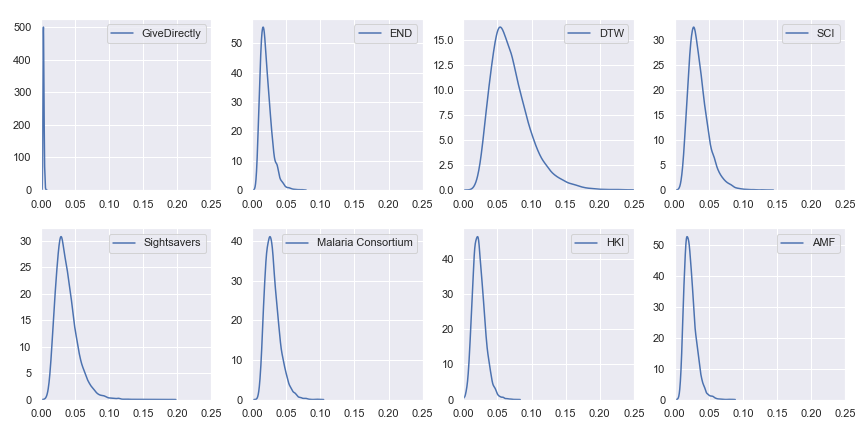
Probability distributions of value per dollar for GiveWell's top charities
For reference, here are the point estimates of value per dollar using GiveWell's values for the charities:
GiveWell's cost-effectiveness estimates for its top charities
| Charity | Value per dollar |
|---|---|
| GiveDirectly | 0.0038 |
| The END Fund | 0.0222 |
| Deworm the World | 0.0738 |
| Schistosomiasis Control Initiative | 0.0378 |
| Sightsavers | 0.0394 |
| Malaria Consortium | 0.0326 |
| Helen Keller International | 0.0223 |
| Against Malaria Foundation | 0.0247 |
I've also plotted a version in which the results are normalized—I divided the results for each charity by that charity's expected value per dollar. Instead of showing the probability distribution on the value per dollar for each charity, this normalized version shows the probability distribution on the percentage of that charity's expected value that it achieves. This version of the plot abstracts from the actual value per dollar and emphasizes the spread of uncertainty. It also reëmphasizes the earlier point that—because we use the same spread of uncertainty for each input parameter—the current results are telling us more about the structure of the model than about the world. For real results, go try the Jupyter notebook!
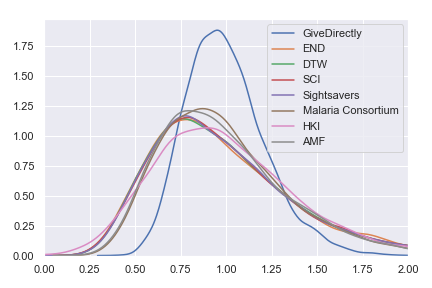
Probability distributions for percentage of expected value obtained with each of GiveWell's top charities
Section recap
Our preliminary conclusion is that all of GiveWell's top charities cost-effectiveness estimates have similar uncertainty with GiveDirectly being a bit more certain than the rest. However, this is mostly an artifact of pretending that we are exactly equally uncertain about each input parameter.
Sensitivity analysis of GiveWell's cost effectiveness estimates
Section overview
In the previous section, we introduced GiveWell's cost-effectiveness analysis which uses a spreadsheet model to take point estimates of uncertain input parameters to point estimates of uncertain results. We adjusted this approach to take probability distributions on the input parameters and in exchange got probability distributions on the resulting cost-effectiveness estimates. But this machinery lets us do more. Now that we've completed an uncertainty analysis, we can move on to sensitivity analysis.
The basic idea of sensitivity analysis is, when working with uncertain values, to see which input values most affect the output when they vary. For example, if you have the equation and each of and varies uniformly over the range from 5 to 10, is much more sensitive to then . A sensitivity analysis is practically useful in that it can offer you guidance as to which parameters in your model it would be most useful to investigate further (i.e. to narrow their uncertainty).
Visual (scatter plot) and delta moment-independent sensitivity analysis on GiveWell's cost-effectiveness models show which input parameters the cost-effectiveness estimates are most sensitive to. Preliminary results (given our input uncertainty) show that some input parameters are much more influential on the final cost-effectiveness estimates for each charity than others.
Visual sensitivity analysis
The first kind of sensitivity analysis we'll run is just to look at scatter plots comparing each input parameter to the final cost-effectiveness estimates. We can imagine these scatter plots as the result of running the following procedure many times[4]: sample a single value from the probability distribution for each input parameter and run the calculation on these values to determine a result value. If we repeat this procedure enough times, it starts to approximate the true values of the probability distributions.
(One nice feature of this sort of analysis is that we see how the output depends on a particular input even in the face of variations in all the other inputs—we don't hold everything else constant. In other words, this is a global sensitivity analysis.)
(Caveat: We are again pretending that we are equally uncertain about each input parameter and the results reflect this limitation. To see the analysis result for different input uncertainties, edit and run the Jupyter notebook.)
Direct cash transfers
GiveDirectly
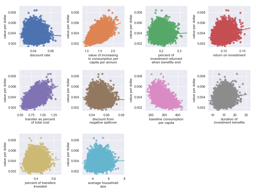
Scatter plots showing sensitivity of GiveDirectly's cost-effectiveness to each input parameter
The scatter plots show that, given our choice of input uncertainty, the output is most sensitive (i.e. the scatter plot for these parameters shows the greatest directionality) to the input parameters:
Highlighted input factors to which result is highly sensitive
| Input | Type of uncertainty | Meaning/importance |
|---|---|---|
| value of increasing ln consumption per capita per annum | Moral | Determines final conversion between empirical outcomes and value |
| transfer as percent of total cost | Operational | Determines cost of results |
| return on investment | Opportunities available to recipients | Determines stream of consumption over time |
| baseline consumption per capita | Empirical | Diminishing marginal returns to consumption mean that baseline consumption matters |
Deworming
Some useful and non-obvious context for the following is that the primary putative benefit of deworming is increased income later in life.
The END Fund
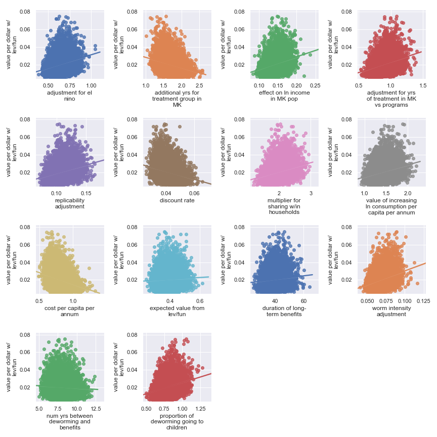
Scatter plots showing sensitivity of the END Fund's cost-effectiveness to each input parameter
Here, it's a little harder to identify certain factors as more important. It seems that the final estimate is (given our input uncertainty) the result of many factors of medium effect. It does seem plausible that the output is somewhat less sensitive to these factors:
Highlighted input factors to which result is minimally sensitive
| Input | Type of uncertainty | Meaning/(un)importance |
|---|---|---|
| num yrs between deworming and benefits | Forecast | Affects how much discounting of future income streams must be done |
| duration of long-term benefits | Forecast | The length of time for a which a person works and earns income |
| expected value from leverage and funging | Game theoretic | How much does money donated to the END Fund shift around other money |
Deworm the World
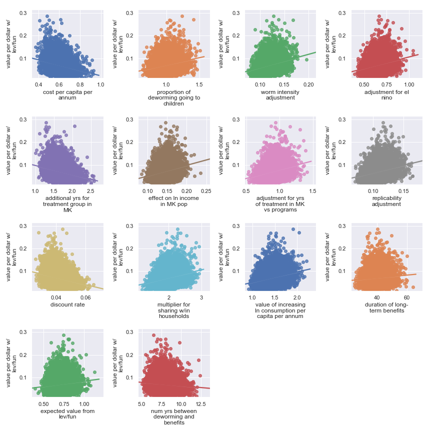
Scatter plots showing sensitivity of the Deworm the World's cost-effectiveness to each input parameter
Again, it's a little harder to identify certain factors as more important. It seems that the final estimate is (given our input uncertainty) the result of many factors of medium effect. It does seem plausible that the output is somewhat less sensitive to these factors:
Highlighted input factors to which result is minimally sensitive
| Input | Type of uncertainty | Meaning/(un)importance |
|---|---|---|
| num yrs between deworming and benefits | Forecast | Affects how much discounting of future income streams must be done |
| duration of long-term benefits | Forecast | The length of time for a which a person works and earns income |
| expected value from leverage and funging | Game theoretic | How much does money donated to Deworm the World shift around other money |
Schistosomiasis Control Initiative
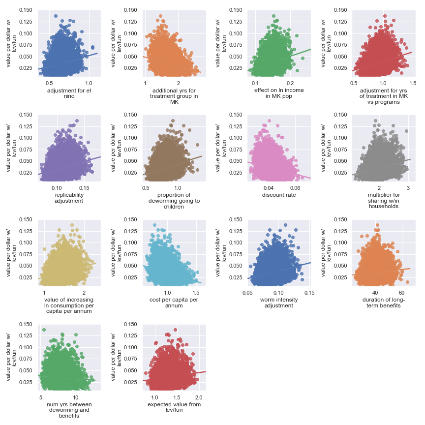
Scatter plots showing sensitivity of the Schistosomiasis Control Initiative's cost-effectiveness to each input parameter
Again, it's a little harder to identify certain factors as more important. It seems that the final estimate is (given our input uncertainty) the result of many factors of medium effect. It does seem plausible that the output is somewhat less sensitive to these factors:
Highlighted input factors to which result is minimally sensitive
| Input | Type of uncertainty | Meaning/(un)importance |
|---|---|---|
| num yrs between deworming and benefits | Forecast | Affects how much discounting of future income streams must be done |
| duration of long-term benefits | Forecast | The length of time for a which a person works and earns income |
| expected value from leverage and funging | Game theoretic | How much does money donated to Schistosomiasis Control Initiative shift around other money |
Sightsavers
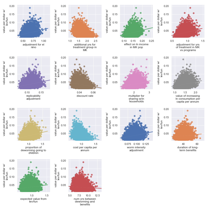
Scatter plots showing sensitivity of the Sightsavers' cost-effectiveness to each input parameter
Again, it's a little harder to identify certain factors as more important. It seems that the final estimate is (given our input uncertainty) the result of many factors of medium effect. It does seem plausible that the output is somewhat less sensitive to these factors:
Highlighted input factors to which result is minimally sensitive
| Input | Type of uncertainty | Meaning/(un)importance |
|---|---|---|
| num yrs between deworming and benefits | Forecast | Affects how much discounting of future income streams must be done |
| duration of long-term benefits | Forecast | The length of time for a which a person works and earns income |
| expected value from leverage and funging | Game theoretic | How much does money donated to Sightsavers shift around other money |
Seasonal malaria chemoprevention
Malaria Consortium
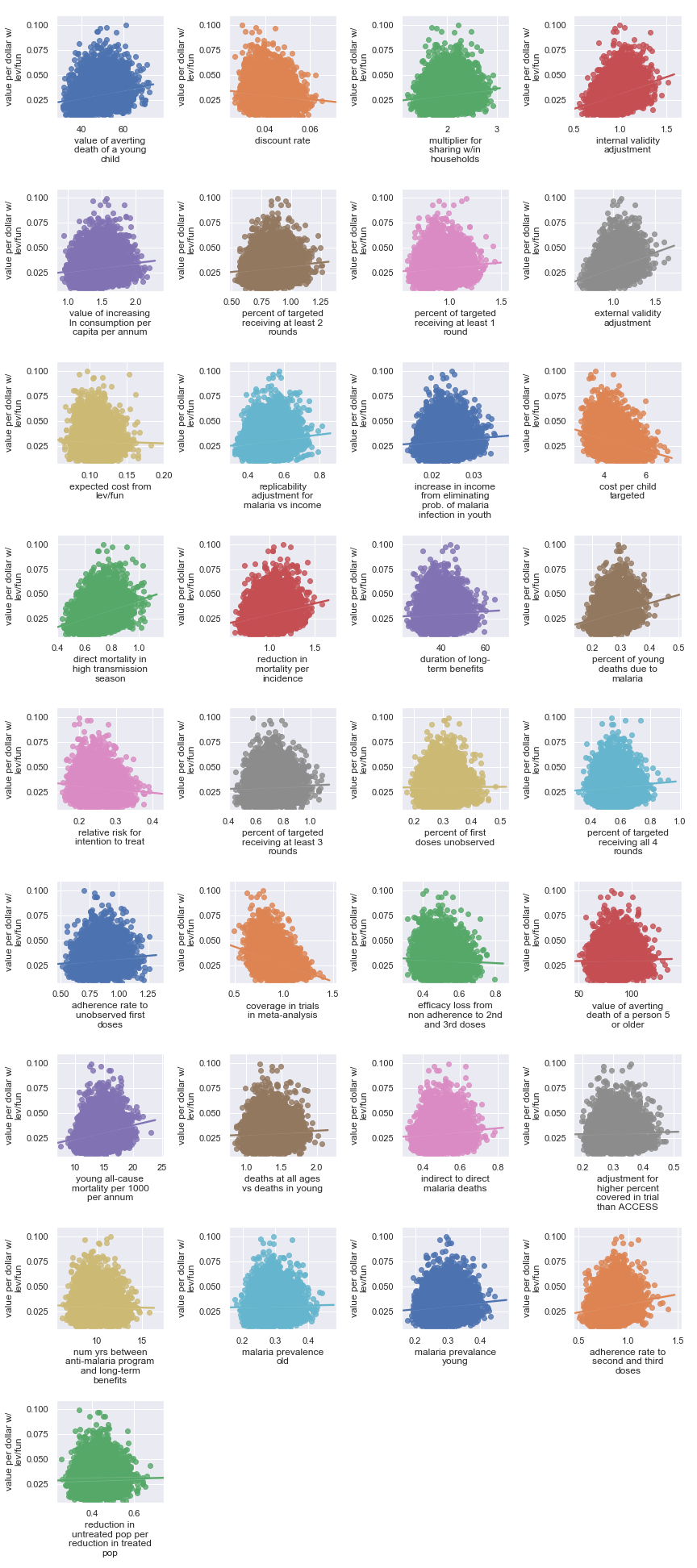
Scatter plots showing sensitivity of Malaria Consortium's cost-effectiveness to each input parameter
The scatter plots show that, given our choice of input uncertainty, the output is most sensitive (i.e. the scatter plot for these parameters shows the greatest directionality) to the input parameters:
Highlighted input factors to which result is highly sensitive
| Input | Type of uncertainty | Meaning/importance |
|---|---|---|
| direct mortality in high transmission season | Empirical | Fraction of overall malaria mortality during the peak transmission season and amenable to SMC |
| internal validity adjustment | Methodological | How much do we trust the results of the underlying SMC studies |
| external validity adjustment | Methodological | How much do the results of the underlying SMC studies transfer to new settings |
| coverage in trials in meta-analysis | Historical/methodological | Determines how much coverage an SMC program needs to achieve to match studies |
| value of averting death of a young child | Moral | Determines final conversion between empirical outcomes and value |
| cost per child targeted | Operational | Affects cost of results |
Vitamin A supplementation
Helen Keller International
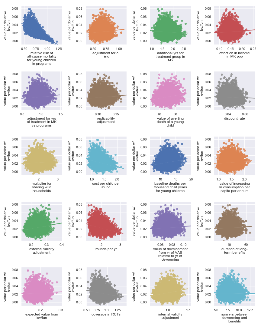
Scatter plots showing sensitivity of the Helen Keller International's cost-effectiveness to each input parameter
The scatter plots show that, given our choice of input uncertainty, the output is most sensitive to the input parameters:
Highlighted input factors to which result is highly sensitive
| Input | Type of uncertainty | Meaning/importance |
|---|---|---|
| relative risk of all-cause mortality for young children in programs | Causal | How much do VAS programs affect mortality |
| cost per child per round | Operational | Affects cost of results |
| rounds per year | Operational | Affects cost of results |
Bednets
Against Malaria Foundation
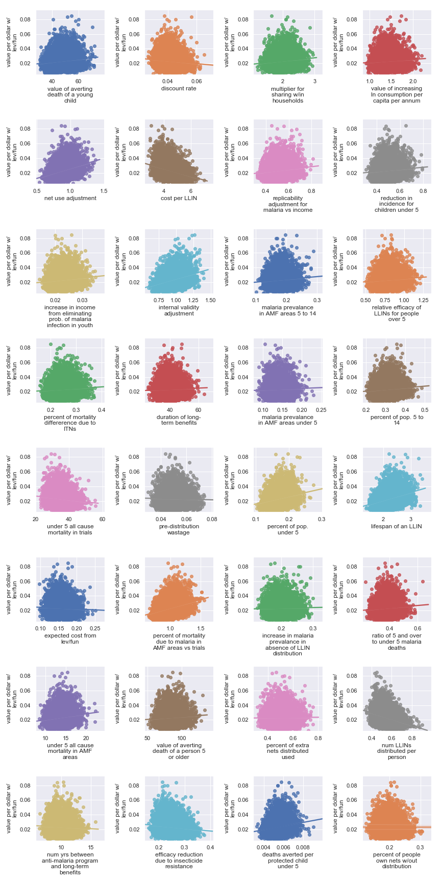
Scatter plots showing sensitivity of Against Malaria Foundation's cost-effectiveness to each input parameter
The scatter plots show that, given our choice of input uncertainty, the output is most sensitive (i.e. the scatter plot for these parameters shows the greatest directionality) to the input parameters:
Highlighted input factors to which result is highly sensitive
| Input | Type of uncertainty | Meaning/importance |
|---|---|---|
| num LLINs distributed per person | Operational | Affects cost of results |
| cost per LLIN | Operational | Affects cost of results |
| deaths averted per protected child under 5 | Causal | How effective is the core activity |
| lifespan of an LLIN | Empirical | Determines how many years of benefit accrue to each distribution |
| net use adjustment | Empirical | Determines benefits from LLIN as mediated by proper and improper use |
| internal validity adjustment | Methodological | How much do we trust the results of the underlying studies |
| percent of mortality due to malaria in AMF areas vs trials | Empirical/historical | Affects size of the problem |
| percent of pop. under 5 | Empirical | Affects size of the problem |
Delta moment-independent sensitivity analysis
If eyeballing plots seems a bit unsatisfying to you as a method for judging sensitivity, not to worry. We also have the results of a more formal sensitivity analysis. This method is called delta moment-independent sensitivity analysis.
(the delta moment-independent sensitivity indicator of parameter ) "represents the normalized expected shift in the distribution of [the output] provoked by [that input]". To make this meaning more explicit, we'll start with some notation/definitions. Let:
- be the random variables used as input parameters
- so that is a function from to describing the relationship between inputs and outputs—i.e. GiveWell's cost-effectiveness model
- be the density function of the result —i.e. the probability distributions we've already seen showing the cost-effectiveness for each charity
- be the conditional density of Y with one of the parameters fixed—i.e. a probability distribution for the cost-effectiveness of a charity while pretending that we know one of the input values precisely
With these in place, we can define . It is:
.
The inner can be interpreted as the total area between probability density function and probability density function . This is the "shift in the distribution of provoked by " we mentioned earlier. Overall, then says:
- pick one value for and measure the shift in the output distribution from the "default" output distribution
- do that for each possible and take the expectation
Some useful properties to point out:
- ranges from 0 to 1
- If the output is independent of the input, for that input is 0
- The sum of for each input considered separately isn't necessarily 1 because there can be interaction effects
In the plots below, for each charity, we visualize the delta sensitivity (and our uncertainty about that sensitivity) for each input parameter.
Direct cash transfers
GiveDirectly
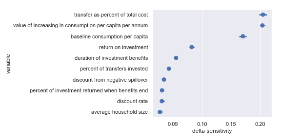
Delta sensitivities for each input parameter in the GiveDirectly cost-effectiveness calculation
Comfortingly, this agrees with the results of our scatter plot sensitivity analysis. For convenience, I have copied the table from the scatter plot analysis describing the most influential inputs:
Highlighted input factors to which result is highly sensitive
| Input | Type of uncertainty | Meaning/importance |
|---|---|---|
| value of increasing ln consumption per capita per annum | Moral | Determines final conversion between outcomes and value |
| transfer as percent of total cost | Operational | Affects cost of results |
| return on investment | Opportunities available to recipients | Determines stream of consumption over time |
| baseline consumption per capita | Empirical | Diminishing marginal returns to consumption mean that baseline consumption matters |
Deworming
The END Fund
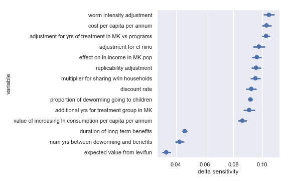
Delta sensitivities for each input parameter in the END Fund cost-effectiveness calculation
Comfortingly, this again agrees with the results of our scatter plot sensitivity analysis[5]. For convenience, I have copied the table from the scatter plot analysis describing the least influential inputs:
Highlighted input factors to which result is minimally sensitive
| Input | Type of uncertainty | Meaning/(un)importance |
|---|---|---|
| num yrs between deworming and benefits | Forecast | Affects how much discounting of future income streams must be done |
| duration of long-term benefits | Forecast | The length of time for a which a person works and earns income |
| expected value from leverage and funging | Game theoretic | How much does money donated to the END Fund shift around other money |
Deworm the World
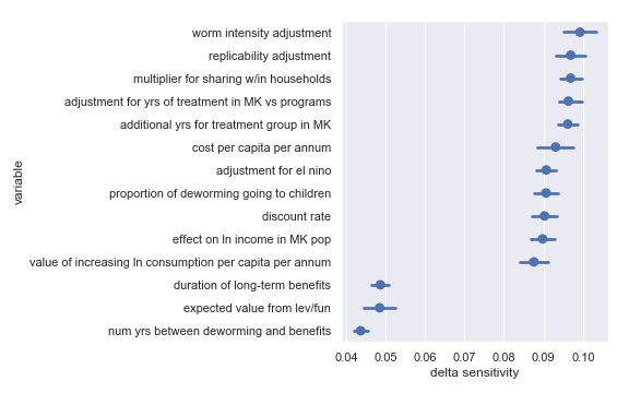
Delta sensitivities for each input parameter in the Deworm the World cost-effectiveness calculation
For convenience, I have copied the table from the scatter plot analysis describing the least influential inputs:
Highlighted input factors to which result is minimally sensitive
| Input | Type of uncertainty | Meaning/(un)importance |
|---|---|---|
| num yrs between deworming and benefits | Forecast | Affects how much discounting of future income streams must be done |
| duration of long-term benefits | Forecast | The length of time for a which a person works and earns income |
| expected value from leverage and funging | Game theoretic | How much does money donated to Deworm the World shift around other money |
Schistosomiasis Control Initiative
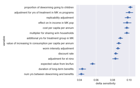
Delta sensitivities for each input parameter in the Schistosomiasis Control Initiative cost-effectiveness calculation
For convenience, I have copied the table from the scatter plot analysis describing the least influential inputs:
Highlighted input factors to which result is minimally sensitive
| Input | Type of uncertainty | Meaning/(un)importance |
|---|---|---|
| num yrs between deworming and benefits | Forecast | Affects how much discounting of future income streams must be done |
| duration of long-term benefits | Forecast | The length of time for a which a person works and earns income |
| expected value from leverage and funging | Game theoretic | How much does money donated to Schistosomiasis Control Initiative shift around other money |
Sightsavers
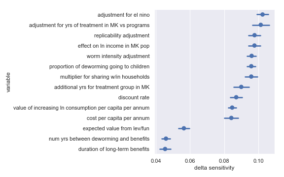
Delta sensitivities for each input parameter in the Sightsavers cost-effectiveness calculation
For convenience, I have copied the table from the scatter plot analysis describing the least influential inputs:
Highlighted input factors to which result is minimally sensitive
| Input | Type of uncertainty | Meaning/(un)importance |
|---|---|---|
| num yrs between deworming and benefits | Forecast | Affects how much discounting of future income streams must be done |
| duration of long-term benefits | Forecast | The length of time for a which a person works and earns income |
| expected value from leverage and funging | Game theoretic | How much does money donated to Sightsavers shift around other money |
Deworming comment
That we get substantially identical results in terms of delta sensitivities for each deworming charity is not surprising: The structure of each calculation is the same and (for the sake of not tainting the analysis with my idiosyncratic perspective) the uncertainty on each input parameter is the same.
Seasonal malaria chemoprevention
Malaria Consortium
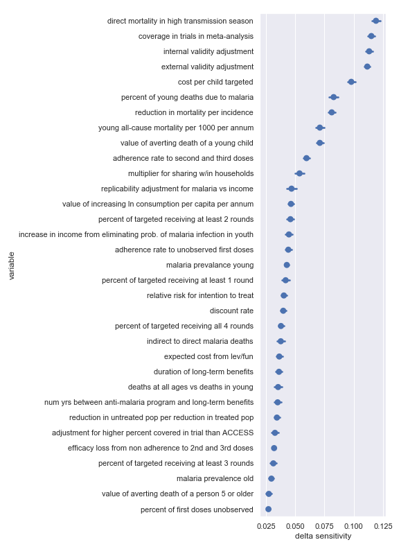
Delta sensitivities for each input parameter in the Malaria Consortium cost-effectiveness calculation
Again, there seems to be good agreement between the delta sensitivity analysis and the scatter plot sensitivity analysis though there is perhaps a bit of reordering in the top factor. For convenience, I have copied the table from the scatter plot analysis describing the most influential inputs:
Highlighted input factors to which result is highly sensitive
| Input | Type of uncertainty | Meaning/importance |
|---|---|---|
| internal validity adjustment | Methodological | How much do we trust the results of the underlying SMC studies) |
| direct mortality in high transmission season | Empirical | Fraction of overall malaria mortality during the peak transmission season and amenable to SMC |
| cost per child targeted | Operational | Afffects cost of results |
| external validity adjustment | Methodological | How much do the results of the underlying SMC studies transfer to new settings |
| coverage in trials in meta-analysis | Historical/methodological | Determines how much coverage an SMC program needs to achieve to match studies |
| value of averting death of a young child | Moral | Determines final conversion between outcomes and value |
Vitamin A supplementation
Hellen Keller International
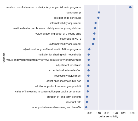
Delta sensitivities for each input parameter in the Helen Keller International cost-effectiveness calculation
Again, there's broad agreement between the scatter plot analysis and this one. This analysis perhaps makes the crucial importance of the relative risk of all-cause mortality for young children in VAS programs even more obvious. For convenience, I have copied the table from the scatter plot analysis describing the most influential inputs:
Highlighted input factors to which result is highly sensitive
| Input | Type of uncertainty | Meaning/importance |
|---|---|---|
| relative risk of all-cause mortality for young children in programs | Causal | How much do VAS programs affect mortality |
| cost per child per round | Operational | Affects the total cost required to achieve effect |
| rounds per year | Operational | Affects the total cost required to achieve effect |
Bednets
Against Malaria Foundation
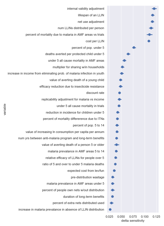
Delta sensitivities for each input parameter in the Against Malaria Foundation cost-effectiveness calculation
Again, there's broad agreement between the scatter plot analysis and this one. For convenience, I have copied the table from the scatter plot analysis describing the most influential inputs:
Highlighted input factors to which result is highly sensitive
| Input | Type of uncertainty | Meaning/importance |
|---|---|---|
| num LLINs distributed per person | Operational | Affects the total cost required to achieve effect |
| cost per LLIN | Operational | Affects the total cost required to achieve effect |
| deaths averted per protected child under 5 | Causal | How effective is the core activity |
| lifespan of an LLIN | Empirical | Determines how many years of benefit accrue to each distribution |
| net use adjustment | Empirical | Affects benefits from LLIN as mediated by proper and improper use |
| internal validity adjustment | Methodological | How much do we trust the results of the underlying studies |
| percent of mortality due to malaria in AMF areas vs trials | Empirical/historical | Affects size of the problem |
| percent of pop. under 5 | Empirical | Affects size of the problem |
Section recap
We performed visual (scatter plot) sensitivity analyses and delta moment-independent sensitivity analyses on GiveWell's top charities. Conveniently, these two methods generally agreed as to which input factors had the biggest influence on the output. For each charity, we found that there were clear differences in the sensitivity indicators for different inputs.
This suggests that certain inputs are better targets than others for uncertainty reduction. For example, the overall estimate of the cost-effectiveness of Helen Keller International's vitamin A supplementation program depends much more on the relative risk of all-cause mortality for children in VAS programs than it does on the expected value from leverage and funging. If the cost of investigating each were the same, it would be better to spend time on the former.
An important caveat to remember is that these results still reflect my fairly arbitrary (but scrupulously neutral) decision to pretend that we equally uncertain about each input parameter. To remedy this flaw, head over to the Jupyter notebook and tweak the input distributions.
Uncertainty and sensitivity analysis of GiveWell's ranking
Section overview
In the last two sections, we performed uncertainty and sensitivity analyses on GiveWell's charity cost-effectiveness estimates. Our outputs were, respectively:
- probability distributions describing our uncertainty about the value per dollar obtained for each charity and
- estimates of how sensitive each charity's cost-effectiveness is to each of its input parameters
One problem with this is that we are not supposed to take the cost-effectiveness estimates literally. Arguably, the real purpose of GiveWell's analysis is not to produce exact numbers but to assess the relative quality of each charity evaluated.
Another issue is that by treating each cost-effectiveness estimate as independent we underweight parameters which are shared across many models. For example, the moral weight that ought to be assigned to increasing consumption shows up in many models. If we consider all the charity-specific models together, this input seems to become more important.
Our solution to these problems will be to use distance metrics on the overall charity rankings. By using distance metrics across these multidimensional outputs, we can perform uncertainty and sensitivity analysis to answer questions about:
- how uncertain we are about the overall relative cost-effectiveness of the charities
- which input parameters this overall relative cost-effectiveness is most sensitive to
Metrics on rankings
Our first step on the path to a solution is to abstract away from particular values in the cost-effectiveness analysis and look at the overall rankings returned. That is we want to transform:
GiveWell's cost-effectiveness estimates for its top charities
| Charity | Value per $10,000 donated |
|---|---|
| GiveDirectly | 38 |
| The END Fund | 222 |
| Deworm the World | 738 |
| Schistosomiasis Control Initiative | 378 |
| Sightsavers | 394 |
| Malaria Consortium | 326 |
| Against Malaria Foundation | 247 |
| Helen Keller International | 223 |
into:
Givewell's top charities ranked from most cost-effective to least
- Deworm the World
- Sightsavers
- Schistosomiasis Control Initiative
- Malaria Consortium
- Against Malaria Foundation
- Helen Keller International
- The END Fund
- GiveDirectly
But how do we usefully express probabilities over rankings[6] (rather than probabilities over simple cost-effectivness numbers)? The approach we'll follow below is to characterize a ranking produced by a run of the model by computing its distance from the reference ranking listed above (i.e. GiveWell's current best estimate). Our output probability distribution will then express how far we expect to be from the reference ranking—how much we might learn about the ranking with more information on the inputs. For example, if the distribution is narrow and near 0, that means our uncertain input parameters mostly produce results similar to the reference ranking. If the distribution is wide and far from 0, that means our uncertain input parameters produce results that are highly uncertain and not necessarily similar to the reference ranking.
Spearman's footrule
What is this mysterious distance metric between rankings that enables the above approach? One such metric is called Spearman's footrule distance. It's defined as:
where:
- and are rankings,
- varies over all the elements of the rankings and
- returns the integer position of item in ranking .
In other words, the footrule distance between two rankings is the sum over all items of the (absolute) difference in positions for each item. (We also add a normalization factor so that the distance varies ranges from 0 to 1 but omit that trivia here.)
So the distance between A, B, C and A, B, C is 0; the (unnormalized) distance between A, B, C and C, B, A is 4; and the (unnormalized) distance between A, B, C and B, A, C is 2.
Kendall's tau
Another common distance metric between rankings is Kendall's tau. It's defined as:
where:
- and are again rankings,
- and are items in the set of unordered pairs of distinct elements in and
- if and are in the same order (concordant) in and and otherwise (discordant)
In other words, the Kendall tau distance looks at all possible pairs across items in the rankings and counts up the ones where the two rankings disagree on the ordering of these items. (There's also a normalization factor that we've again omitted so that the distance ranges from 0 to 1.)
So the distance between A, B, C and A, B, C is 0; the (unnormalized) distance between A, B, C and C, B, A is 3; and the (unnormalized) distance between A, B, C and B, A, C is 1.
Angular distance
One drawback of the above metrics is that they throw away information in going from the table with cost-effectiveness estimates to a simple ranking. What would be ideal is to keep that information and find some other distance metric that still emphasizes the relationship between the various numbers rather than their precise values.
Angular distance is a metric which satisfies these criteria. We can regard the table of charities and cost-effectiveness values as an 8-dimensional vector. When our output produces another vector of cost-effectiveness estimates (one for each charity), we can compare this to our reference vector by finding the angle between the two[7].
Results
Uncertainties
To recap, what we're about to see next is the result of running our model many times with different sampled input values. In each run, we compute the cost-effectiveness estimates for each charity and compare those estimates to the reference ranking (GiveWell's best estimate) using each of the tau, footrule and angular distance metrics. Again, the plots below are from running the analysis while pretending that we're equally uncertain about each input parameter. To avoid this limitation, go to the Jupyter notebook and adjust the input distributions.
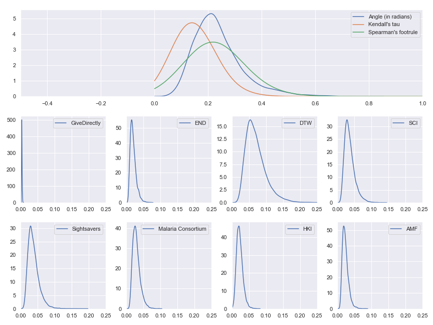
Probability distributions of value per dollar for each of GiveWell's top charity and probability distributions for the distance between model results and the reference results
We see that our input uncertainty does matter even for these highest level results—there are some input values which cause the ordering of best charities to change. If the gaps between the cost-effectiveness estimates had been very large or our input uncertainty had been very small, we would have expected essentially all of the probability mass to be concentrated at 0 because no change in inputs would have been enough to meaningfully change the relative cost-effectiveness of the charities.
Visual sensitivity analysis
We can now repeat our visual sensitivity analysis but using our distance metrics from the reference as our outcome of interest instead of individual cost-effectiveness estimates. What these plots show is how sensitive the relative cost-effectiveness of the different charities is to each of the input parameters used in any of the cost-effectiveness models (so, yes, there are a lot of parameters/plots). We have three big plots, one for each distance metric—footrule, tau and angle. In each plot, there's a subplot corresponding to each input factor used anywhere in the GiveWell's cost-effectiveness analysis.
Scatter plots showing sensitivity of the footrule distance with respect to each input parameter

Scatter plots showing sensitivity of the tau distance with respect to each input parameter

Scatter plots showing sensitivity of the angular distance with respect to each input parameter

(The banding in the tau and footrule plots is just an artifact of those distance metrics returning integers (before normalization) rather than reals.)
These results might be a bit surprising at first. Why are there so many charity-specific factors with apparently high sensitivity indicators? Shouldn't input parameters which affect all models have the biggest influence on the overall result? Also, why do so few of the factors that showed up as most influential in the charity-specific sensitivity analyses from last section make it to the top?
However, after reflecting for a bit, this makes sense. Because we're interested in the relative performance of the charities, any factor which affects them all equally is of little importance here. Instead, we want factors that have a strong influence on only a few charities. When we go back to the earlier charity-by-charity sensitivity analysis, we see that many of the input parameters we identified as most influential where shared across charities (especially across the deworming charities). Non-shared factors that made it to the top of the charity-by-charity lists—like the relative risk of all-cause mortality for young children in VAS programs—show up somewhat high here too.
But it's hard to eyeball the sensitivity when there are so many factors and most are of small effect. So let's quickly move on to the delta analysis.
Delta moment-independent sensitivity analysis
Again, we'll have three big plots, one for each distance metric—footrule, tau and angle. In each plot, there's an estimate of the delta moment-independent sensitivity for each input factor used anywhere in the GiveWell's cost-effectiveness analysis (and an indication of how confident that sensitivity estimate is).
Delta sensitivities for each input parameter in footrule distance analysis

Delta sensitivities for each input parameter in the tau distance analysis

Delta sensitivities for each input parameter in angular distance analysis

So these delta sensitivities corroborate the suspicion that arose during the visual sensitivity analysis—charity-specific input parameters have the highest sensitivity indicators.
The other noteworthy result is which charity-specific factors are the most influential depends somewhat on which distance metric we use. The two rank-based metrics—tau and footrule distance—both suggest that the final charity ranking (given these inputs) is most sensitive to the worm intensity adjustment and cost per capita per annum of Sightsavers and the END Fund. These input parameters are a bit further down (though still fairly high) in the list according to the angular distance metric.
Needs more meta
It would be nice to check that our distance metrics don't produce totally contradictory results. How can we accomplish this? Well, the plots above already order the input factors according to their sensitivity indicators... That means we have rankings of the sensitivities of the input factors and we can compare the rankings using Kendall's tau and Spearman's footrule distance. If that sounds confusing hopefully the table clears things up:
Using Kendall's tau and Spearman's footrule distance to assess the similarity of sensitivity rankings generated under different distance metrics
| Delta sensitivity rankings compared | Tau distance | Footrule distance |
|---|---|---|
| Tau and footrule | 0.358 | 0.469 |
| Tau and angle | 0.365 | 0.516 |
| Angle and footrule | 0.430 | 0.596 |
So it looks like the three rankings have middling agreement. Sensitivities according to tau and footrule agree the most while sensitivities according to angle and footrule agree the least. The disagreement probably also reflects random noise since the confidence intervals for many of the variables' sensitivity indicators overlap. We could presumably shrink these confidence intervals and reduce the noise by increasing the number of samples used during our analysis.
To the extent that the disagreement isn't just noise, it's not entirely surprising—part of the point of using different distance metrics is to capture different notions of distance, each of which might be more or less suitable for a given purpose. But the divergence does mean that we'll need to carefully pick which metric to pay attention to depending on the precise questions we're trying to answer. For example, if we just want to pick the single top charity and donate all our money to that, factors with high sensitivity indicators according to footrule distance might be the most important to pin down. On the other hand, if we want to distribute our money in proportion to each charity's estimated cost-effectiveness, angular distance is perhaps a better metric to guide our investigations.
Section recap
We started with a couple of problems with our previous analysis: we were taking cost-effectiveness estimates literally and looking at them independently instead of as parts of a cohesive analysis. We addressed these problems by redoing our analysis while looking at distance from the current best cost-effectiveness estimates. We found that our input uncertainty is consequential even when looking only at the relative cost-effectiveness of the charities. We also found that input parameters which are important but unique to a particular charity often affect the final relative cost-effectiveness substantially.
Finally, we have the same caveat as last time: these results still reflect my fairly arbitrary (but scrupulously neutral) decision to pretend that we equally uncertain about each input parameter. To remedy this flaw and get results which are actually meaningful, head over to the Jupyter notebook and tweak the input distributions.
Recap
GiveWell models the cost-effectiveness of its top charities with point estimates in a spreadsheet. We insisted that working with probability distributions instead of point estimates more fully reflects our state of knowledge. By performing uncertainty analysis, we got a better sense of how uncertain the results are (e.g. GiveDirectly is the most certain given our inputs). After uncertainty analysis, we proceeded to sensitivity analysis and found that indeed there were some input parameters that were more influential than others. The most influential parameters are likely targets for further investigation and refinement. The final step we took was to combine the individual charity cost-effectiveness estimates into one giant model. By looking at how far (using three different distance metrics) these results deviated from the current overall cost-effectiveness analysis, we accomplished two things. First, we confirmed that our input uncertainty is indeed consequential—there are some plausible input values which might reorder the top charities in terms of cost-effectiveness. Second, we identified which input parameters (given our uncertainty) have the highest sensitivity indicators and therefore are the best targets for further scrutiny. We also found that this final sensitivity analysis was fairly sensitive to which distance metric we use so it's important to pick a distance metric tailored to the question of interest.
Finally, throughout, I reminded you that this is more of a template for an analysis than an actual analysis because we pretended to be equally uncertain about each input parameter. To get a more useful analysis, you'll have to edit the input uncertainty to reflect your actual beliefs and run the Jupyter notebook.
Appendix
Sobol indices for per-charity cost-effectiveness
I also did a variance-based sensitivity analysis with Sobol indices. Those plots follow.
The variable order in each plot is from the input parameter with the highest sensitivity to the input parameter with the lowest sensitivity. That makes it straightforward to compare the ordering of sensitivities according to the delta moment-independent method and according to the Sobol method. We see that there is broad—but not perfect—agreement between the methods.
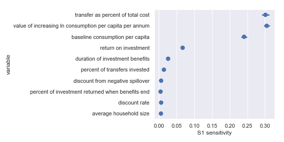
Sobol sensitivities for each input parameter in the GiveDirectly cost-effectiveness calculation
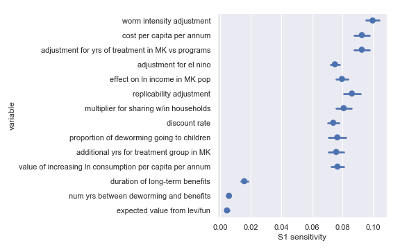
Sobol sensitivities for each input parameter in the END Fund cost-effectiveness calculation
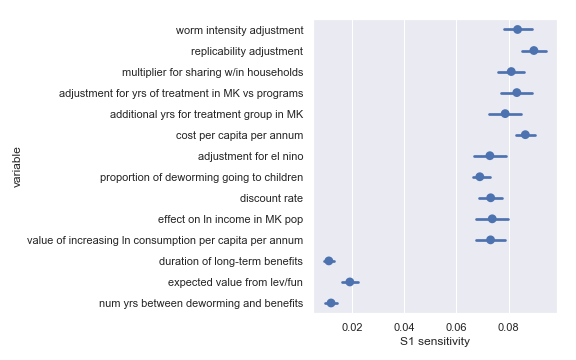
Sobol sensitivities for each input parameter in the Deworm the World cost-effectiveness calculation

Sobol sensitivities for each input parameter in the Schistosomiasis Control Initiative cost-effectiveness calculation
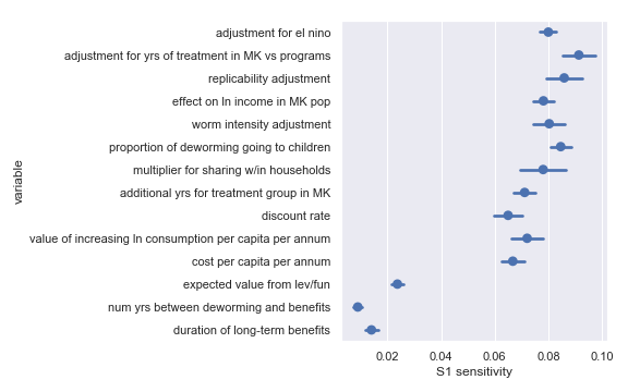
Sobol sensitivities for each input parameter in the Sightsavers cost-effectiveness calculation
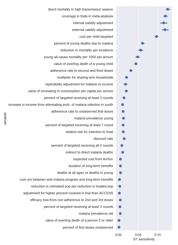
Sobol sensitivities for each input parameter in the Malaria Consortium cost-effectiveness calculation
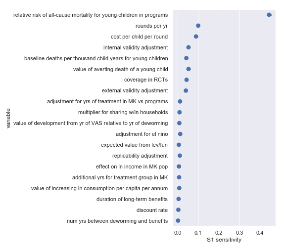
Sobol sensitivities for each input parameter in the Helen Keller International cost-effectiveness calculation
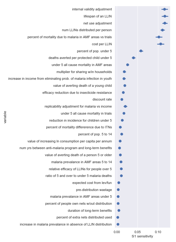
Sobol sensitivities for each input parameter in the Against Malaria Foundation cost-effectiveness calculation
Sobol indices for relative cost-effectiveness of charities
The variable order in each plot is from the input parameter with the highest sensitivity to the input parameter with the lowest sensitivity. That makes it straightforward to compare the ordering of sensitivities according to the delta moment-independent method and according to the Sobol method. We see that there is broad—but not perfect—agreement between the different methods.
Sobol sensitivities for each input parameter in footrule distance analysis

Sobol sensitivities for each input parameter in tau distance analysis

Sobol sensitivities for each input parameter in angular distance analysis

Unfortunately, the code implements the 2019 V4 cost-effectiveness analysis instead of the most recent V5 because I just worked off the V4 tab I'd had lurking in my browser for months and didn't think to check for a new version until too late. I also deviated from the spreadsheet in one place because I think there's an error (Update: The error will be fixed in GiveWell's next publically-released version). ↩︎
Log-normal strikes me as a reasonable default distribution for this task: because it's support is (0, +∞) which fits many of our parameters well (they're all positive but some are actually bounded above by 1); and because "A log-normal process is the statistical realization of the multiplicative product of many independent random variables" which also seems reasonable here. ↩︎
When you follow the link, you should see a Jupyter notebook with three "cells". The first is a preamble setting things up. The second has all the parameters with lower and upper bounds. This is the part you want to edit. Once you've edited it, find and click "Runtime > Run all" in the menu. You should eventually see the notebook produce a serious of plots. ↩︎
This is, in fact, approximately what Monte Carlo methods do so this is a very convenient analysis to run. ↩︎
I swear I didn't cheat by just picking the results on the scatter plot that match the delta sensitivities! ↩︎
If we just look at the probability for each possible ranking independently, we'll be overwhelmed by the number of permutations and it will be hard to find any useful structure in our results. ↩︎
The angle between the vectors is a better metric here than the distance between the vectors' endpoints because we're interested in the relative cost-effectiveness of the charities and how those change. If our results show that each charity is twice as effective as in the reference vector, our metric should return a distance of 0 because nothing has changed in the relative cost-effectiveness of each charity. ↩︎

I’d find it useful if you could summarize your main takeaways from the analysis in nontechnical language.
You looked at the overall recap and saw the takeaways there? e.g. Sensitivity analysis indicates that some inputs are substantially more influential than others, and there are some plausible values of inputs which would reorder the ranking of top charities.
These are sort of meta-conclusions though and I'm guessing you're hoping for more direct conclusions. That's sort of hard to do. As I mention in several places, the analysis depends on the uncertainty you feed into it. To maintain "neutrality", I just pretended to be equally uncertain about each input. But, given this, any simple conclusions like "The AMF cost-effectiveness estimates have the most uncertainty." or "The relative cost-effectiveness is most sensitive to the discount rate." would be misleading at best.
The only way to get simple conclusions like that is to feed input parameters you actually believe in to the linked Jupyter notebook. Or I could put in my best guesses as to inputs and draw simple conclusions from that. But then you'd be learning about me as much as you'd be learning about the world as you see it.
Does that all make sense? Is there another kind of takeaway that you're imagining?
Despite your reservations, I think it would actually be very useful for you to input your best guess inputs (and its likely to be more useful for you to do it than an average EA, given you've thought about this more). My thinking is this. I'm not sure I entirely followed the argument, but I took it that the thrust of what you're saying is "we should do uncertainty analysis (use Monte Carlo simulations instead of point-estimates) as our cost-effectiveness might be sensitive to it". But you haven't shown that GiveWell's estimates are sensitive to a reliance on point estimates (have you?), so you haven't (yet) demonstrated it's worth doing the uncertainty analysis you propose after all. :)
More generally, if someone says "here's a new, really complicated methodology we *could* use", I think its incumbent on them to show that we *should* use it, given the extra effort involved.
Thanks for your thoughts.
Yup, this is the thrust of it.
I think I have---conditionally. The uncertainty analysis shows that, if you think the neutral uncertainty I use as input is an acceptable approximation, substantially different rankings are within the bounds of plausibility. If I put in my own best estimates, the conclusion would still be conditional. It's just that instead of being conditional upon "if you think the neutral uncertainty I use as input is an acceptable approximation" it's conditional upon "if you think my best estimates of the uncertainty are an acceptable approximation".
So the summary point there is that there's really no way to escape conditional conclusions within a subjective Bayesian framework. Conclusions will always be of the form "Conclusion C is true if you accept prior beliefs B". This makes generic, public communication hard (as we're seeing!), but offers lots of benefits too (which I tried to demonstrate in the post---e.g. an explicit quantification of uncertainty, a sense of which inputs are most influential).
If I've given the impression that it's really complicated, I think might have misled. One of the things I really like about the approach is that you pay a relatively modest fixed cost and then you get this kind of analysis "for free". By which I mean the complexity doesn't infect all your actual modeling code. For example, the GiveDirectly model here actually reads more clearly to me than the corresponding spreadsheet because I'm not constantly jumping around trying to figure out what the cell reference (e.g. B23) means in formulas.
Admittedly, some of the stuff about delta moment-independent sensitivity analysis and different distance metrics is a bit more complicated. But the distance metric stuff is specific to this particular problem---not the methodology in general---and the sensitivity analysis can largely be treated as a black box. As long as you understand what the properties of the resulting number are (e.g. ranges from 0-1, 0 means independence), the internal workings aren't crucial.
Given the responses here, I think I will go ahead and try that approach. Though I guess even better would be getting GiveWell's uncertainty on all the inputs (rather than just the inputs highlighted in the "User weights" and "Moral inputs" tab).
Sorry for adding even more text to what's already a lot of text :). Hope that helps.
Did you ever get round to running the analysis with your best guess inputs?
If that revealed substantial decision uncertainty (and especially if you were very uncertain about your inputs), I'd also like to see it run with GiveWell's inputs. They could be aggregated distributions from multiple staff members, elicited using standard methods, or in some cases perhaps 'official' GiveWell consensus distributions. I'm kind of surprised this doesn't seem to have been done already, given obvious issues with using point estimates in non-linear models. Or do you have reason to believe the ranking and cost-effectiveness ratios would not be sensitive to methodological changes like this?
This approach seems to be being neglected by GiveWell, and not taken up by others in this space. (I don't have time to write a full review).
Thanks for this (somewhat overwhelming!) analysis. I tried to do something similar a few years back, and am pretty enthusiastic about the idea of incorporating more uncertainty analysis into cost effectiveness estimates, generally.
One thing (that I don't think you mentioned, though I'm still working through the whole post) this allows you to do is use techniques from Modern Portfolio Theory to create giving portfolios with similar altruistic returns and lower downside risk. I'd be curious to see if your analysis could be used in a similar way.
Oh, very cool! I like the idea of sampling from different GiveWell staffers' values (though I couldn't do that here since I regarded essentially all input parameters as uncertain instead of just the highlighted ones).
I hadn't thought about the MPT connection. I'll think about that more.
@cole_haus: I really like this approach.
One thing that is not clear to me:
I think it's something they should be attuned to, and I'd like to see them go more in the direction of open, transparent, and cleanly-coded models.
By the way I added a few comments and suggestions here and in your blog using hypothes.is, a little browser plugin. I like to do that as you can add comments (even small ones) as highlights/annotations directly in the text
Further opinions/endorsement ...
I think "this approach" (making uncertainty explicit) is important, necessary, and correct...
I'd pair it with "letting the user specify parameters/distributions over moral uncertainty things" (and perhaps even subjective beliefs about different types of evidence).
I think (epistemic basis -- mostly gut feeling) it will likely will make a difference in how charities and interventions rank against each other. At first pass, it may lead to 'basically the same ranking' (or at least, not a strong change). But I suspect that if it is made part of a longer-term careful practice, some things will switch order, and this is meaningful.
It will also enable evaluation of a wider set of charities/interventions. If we make uncertainty explicit, we can feel more comfortable evaluating cases where there is much less empirical evidence.
So I think 'some organization' should be doing this, and I expect this will happen soon; whether that is GiveWell doing it or someone else.
@cole_haus I'm working on a new modeling tool - https://causal.app. If you think it's useful I could try to replicate your analysis with Causal. The advantage would be that the output is an interactive web site where users can play with the assumptions (e.g. plug in different distributions).
If there's another analysis that you think might be a better fit I could also build that. I just think that Causal could be useful for the EA community :)
How did this/how is this going? I'm chatting with Taimur of Causal tomorrow and I wanted to bring this up
How did the chat go?
I wonder if porting GiveWell cost-effectiveness models to causal.app might make them more understandable
He was very positive about it and willing to move forward on it. I didn't/don't have all the bandwidth to follow up as much as I'd like to, but maybe someone else could do. (And I'd hope to turn back to this at some point.)
I think this could be done in addition to and in complement to HazelFire's work. Note that the Hazelfire effort is using squiggle language. I've been following up and encouraging them as well. I hope that we can find a way to leverage the best features of each of these tools, and also bring in domain knowledge.
The link has an extra '.' - https://www.causal.app/
Looks neat, good luck!
Do the expected values of the output probability distributions equal the point estimates that GiveWell gets from their non-probabilistic estimates? If not, how different are they?
More generally, are there any good write-ups about when and how the expected value of a model with multiple random variables differs from the same model filled out with the expected value of each of its random variables?
(I didn't find the answer skimming through, but it might be there already--sorry!)
Short version:
No, but they're close.
Don't know of any write-ups unfortunately, but the linearity of expectation means that the two are equal if and (generally?) only if the model is linear.
Long version:
When I run the Python versions of the models with point estimates, I get:
The (mostly minor) deviations from the official GiveWell numbers are due to:
When I calculate the expected values of the probability distributions given the uniform input uncertainty, I get:
I would generally call these values pretty close.
It's worth noting though that the procedure I used to add uncertainty to inputs doesn't produce inputs distributions that have the original point estimate as their expected value. By creating a 90% CI at ±20% of the original value, the CI is centered around the point estimate but since log normal distributions aren't symmetric, the expected value is not precisely at the the point estimate. That explains some of the discrepancy.
The rest of the discrepancy is presumably from the non-linearity of the models (e.g. there are some logarithms in the models). In general, the linearity of expectation means that the expected value of a linear model of multiple random variables is exactly equal to the linear model of the expected values. For non-linear models, no such rule holds. (The relatively modest discrepancy between the point estimates and the expected values suggests that the models are "mostly" linear.)
Fabulous! This is extremely good to know and it's also quite a relief!
Yes, how does the posterior mode differ from GiveWell's point estimates, and how does this vary as a function of the input uncertainty (confidence interval length)?
(I think my other two recent comments sort of answer each of your questions.)
Thanks for putting this together, it's really interesting! Based on this analysis, it seems the worm wars may have been warranted after all.
I worked on a related project a few years ago, but I was mainly looking for evidence of a "return" to altruistic risk taking. I had a hard time finding impact estimates that quantified their uncertainty, but eventually found a few sources that might interest you. I listed all the standalone sources here, then tried to combine them in a meta-analysis here. I don't have access to most of the underlying models though, so I don't think it's possible to incorporate the results into your sensitivity analysis. I also don't have much of a background in statistics so take the results with a grain of salt.
Some quick points:
More to come!
Nope, it varies. One way you can check this intuitively is: if the discount rate and all other parameters were held constant, we'd have a proper function and our scatter plot would show at most one output value for each input.
There are (at least) two versions I can think of:
Adjust all the input uncertainties in concert. That is, spread all the point estimates by ±20% or all by ±30% , etc. This would be computationally tractable, but I'm not sure it would get us too much extra. I think the key problem with the current approach which would remain is that we're radically more uncertain about some of the inputs than the others.
Adjust all the input uncertainties individually. That is, spread point estimate 1 by ±20%, point estimate 2 by ±10%, etc. Then, spread point estimate 1 by ±10%, spread point estimate 2 by ±20%, etc. Repeat for all combinations of spreads and inputs. This would actually give us somewhat useful information, but would be computational intractable given the number of input parameters.