Primary author: Ishaan Guptasarma, Principal Analyst at SoGive
We recently announced that we will be performing an independent assessment of StrongMinds. This is the first in a series of posts which will culminate in that assessment.
Executive Summary
In order to conduct our review of StrongMinds, we needed to make decisions about how to measure the effectiveness of psychotherapy. The approaches that we considered were mainly:
- An approach used by Happier Lives Institute (HLI), which measures the cumulative effect size of therapy over time (SD-Years) by postulating an initial effect which exponentially decays over time, and integrating under the curve.
- An approach used by some academics, which reports remission rates and number needed to treat (NNT) associated with psychotherapy, and of relapse rates at various time points as reported in longitudinal follow-ups.
We decided that the SD-Years approach used by HLI best captures what we’re trying to capture, because remission, relapse, and NNT use cut-offs which are arbitrary and poorly standardised.
The drawback of this method is that it's based on effect sizes, which can become inflated when ceiling and floor effects artificially reduce the standard deviation. Such artefacts are rarely ever accounted for in meta-analyses and literature that we have encountered.
For each step in our methodology, we've created spreadsheet tools which others can use to quickly check and replicate our work and do further analysis. These tools can do:
- Meta-analysis, for calculating standardised mean differences and aggregating effect sizes across multiple studies to estimate the impact of a therapeutic intervention.
- Linear regressions and meta-regressions, to calculate the rate at which therapeutic effects decay over time.
- Conversion from remission rates and NNTs into effect sizes, and relapse rates into decay rates, and vice versa.
- Conversion of scores between different depression questionnaires.
- Calculation of "standard deviations of improvement" for a single patient, for building intuitions.
About SoGive: SoGive does EA research and supports major donors. If you are a major donor seeking support with your donations, we’d be keen to work with you. Feel free to contact Sanjay on sanjay@sogive.org.
0 Introduction
How should the EA community reason about interventions relating to subjective well being? We typically conceptualise the impact of donating to global health anti-malaria charities in terms of figures such as "£5,000 per child's life saved". While evaluating such estimates is difficult, the fundamental question arguably has a "yes or no" answer: was a child's death averted, or not?
Measuring impact on subjective well being, which is continuous rather than discrete and is typically measured by self-report, requires a different framework. This post explains the dominant frameworks for thinking about this, explores some of the complications that they introduce, and introduces spreadsheet tools for deploying these frameworks. These tools and analytical considerations that will lay the groundwork for subsequent work.
We recommend this post to anyone interested in doing analysis on mental health. It may also be useful to anyone doing impact evaluations on continuous phenomena which manifest as unimodal distributions, especially those which might be approximated as normal distributions.
1 The SD-year framework, and why we prefer it to the alternative
Academic studies usually measure the impact of a mental health intervention by using questionnaires to ask how people feel before and after the intervention, and then comparing their scores to a control group which did not receive an intervention. Occasionally, there are follow up studies after some time has elapsed to see how long the effect has lasted over time.
Because there are a large number of questionnaires aimed at measuring mental health, academic reviews of literature need a common metric to summarise data from studies which use different methodologies to survey their participants.
One common method is to decide that, below a given cut-off in a depression questionnaire, the study participant has gone into "remission", which means their depression is considered to have been resolved. By comparing the rate of remission between the intervention and the control group, the "Number Needed to Treat" (NNT), which represents the number of patients you would need to treat before one would be counterfactually cured, can be calculated. Longitudinal data can be incorporated into this framework by looking at the rate at which treated patients ``relapse" (score above the cut-off for depression) over time. An advantage of these methods is that they explain things concretely, in terms of "depressed" vs "not depressed", in a way that may be useful to the way clinicians work. However, different scales use different cut-offs in a way that makes them difficult to directly compare, and morally relevant information about changes that occur outside of the cutoff range is lost.
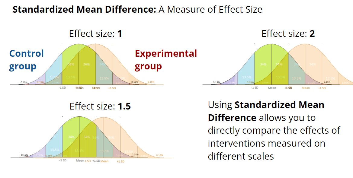
Another method is to report scores of the "treatment group" and the "control group" as means and standard deviations, and use that to calculate the "effect size" as a "standardised mean difference". Academic meta-analyses can aggregate effect sizes from multiple studies to arrive at an overall estimate. However, this traditionally only applied to a single time point. McGuire (2021 a, b) extends this methodology to assess interventions at multiple time points by introducing "SD-Years", a unit which is produced by estimating change in effect size over time and integrating under the curve. To our knowledge, this approach is not widely used elsewhere. We have reviewed this approach used by HLI in their assessment of StrongMinds, and believe it to be superior to the remission/relapse/NNT based framework more commonly used in academic literature.
HLI (and now SoGive) assesses these interventions based on “SD-years”, which captures both:
- The effect size of treatment immediately after therapy, as measured in standard deviations of improvement in depression questionnaire scores.
- The decay of the effects of psychotherapy over time, reflecting the number of years that the positive influence of psychotherapy lasts.
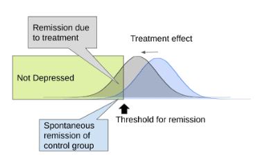
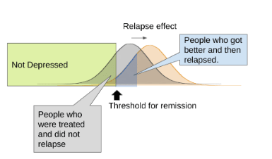
The decay component captures the fact that when the therapy is over, participants may go back to their previous routine and get depressed again. Alternatively, the control group may become less depressed due to some reason unrelated to the intervention - for instance, they might have found therapy or medication through some other avenue, or they may have spontaneously improved on their own.
In order to use the SD-Years framework, it's necessary to understand how to use means and standard deviations to compare raw scores on depression questionnaires, calculate effect sizes, aggregate effect sizes from multiple studies, do linear and meta-regressions to calculate how the effect changes with time and other variables, and convert between effect-size based frameworks and remission/relapse/NNT based frameworks. It's also important to understand the drawbacks of these methods, and catch when they produce misleading results. The remainder of this document contains a series of spreadsheet tools which can accomplish these things, and considerations to be aware of when using these tools. Subsequent analysis will be done using these tools, so that other users can easily audit the results.
2 Tools to calculate SD-years assuming exponential decay
McGuire (2021 a, b) suggests assuming that the benefits of psychotherapy decay exponentially over time. We think that this is a reasonable assumption, which we will comment on further in a later article.
Accordingly, in this model, the two important numbers which determine the impact of psychotherapy are the initial effect size d0 and the decay rate b. Once we have these numbers, we can model how the effect size changes over time using the decay equation:
EffectSize(t) = d0*bt
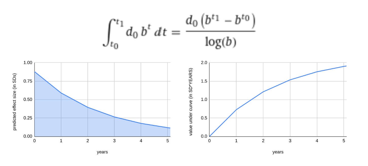
Once the decay equation is established, we can estimate how many "cumulative standard deviations of depression" were averted by integrating the area under the curve.
Left: effect size decaying over time according to the equation EffectSize = d0*bt where d0 is the effect size at time 0, t is time and b is a constant which represents the percent of benefit retained after 1 year if t=1 is a year.
Right: Integration under the curve is used to calculate the morally relevant cumulative benefit over time.
The number produced by this integration is in the units "standard-deviations * time", which we will call SD-years. An intervention which achieves 1 SD-year of impact on depression for one person can be considered to have achieved the equivalent of reducing that person's depression by 1 SD over the time course of one year. Where there are multiple patients, their SD-years can be summed to create an overall metric of impact, which may be assigned a moral weight.
The choice to attach moral weights to SD-years implicitly assume that the following outcomes are of equal value:
- 12 people receiving (1/12) SDs of benefit for one year
- 12 people receiving 1 SD of benefit for one month each
- 1 person receiving 1 SD of benefit for one year
The extent to which we accept this depends on whether we should treat SDs of the underlying scale (e.g. PHQ-9 or some other depression survey) linearly. It also depends on whether we should treat time linearly. In-depth treatment of both of these topics are outside the scope of this article. A subsequent post will discuss how we assign these moral weights.
Estimating effect size decay and cumulative SD years from two or more time points.
The initial effect size d0 and rate of decay b must be empirically determined. If you have depression scores for two or more time points, these values can be determined using linear regression. We've created a toy model so that you can play around with creating models for effect sizes at different time points. See Appendix A for more details about the maths.
Estimating effect size decay using meta-regressions
To empirically determine decay rates from the effect sizes reported in academic literature, it is necessary to do a "meta-regression", which (to oversimplify) one might describe as taking into account that higher powered data points weigh more. Meta-regression was used in McGuire (2021 a, b). We do have a meta regression tool, but at time of publication it is built for linear relationships, and modifying it to model exponential relationships makes it crash if there are any effect sizes below zero, so it's necessary to use other software to do meta-regressions for exponential models with such data.
3 Tools to calculate and aggregate effect sizes
Effect sizes are typically reported as standardised mean differences (SMD), in which the difference between the mean score of the control group and the mean score of the treatment group is divided by a measure of standard deviation which aims to reflect the spread of both groups.
Calculating Standardised Mean Differences
The basic formula to calculate standardised mean differences is
SMD = (𝛍2-𝛍1)/𝜎pooled
Where 𝛍1 and 𝛍2 are the means of the two groups being compared and 𝜎pooled is a measure that combines the standard deviations of the two groups in some manner. Different SMD formulas handle the calculation of 𝜎pooled differently. The best formula is usually Hedges' g, though Glass's ∆ may be more appropriate if one of the two groups is encountering ceiling or floor effects which distort its standard deviation (more on that later). Cohen's d is also commonly used. We've designed user-friendly spreadsheet tools which you can use to calculate SMD effect sizes for any dataset.
Aggregating effect sizes across multiple studies.
Using standardised mean difference is useful because it allows meta-analyses to aggregate the results of different studies which use different survey instruments into a single estimate. This is how almost all the evidence regarding the effect of therapy for depression is reported and aggregated in the academic literature. We've created spreadsheet tools that can aggregate effect sizes across multiple studies. The tools for aggregating effect size were created using the methodology described by Neyeloff (2012).
Using meta-regressions to model how other variables influence effect size
We've also built a tool that can do meta-regressions for the association between effect sizes and another variable. Given a set of effect sizes, variances, and a third factor, the tool can tell you the linear equation that best describes the relationship between the effect size and the third factor. This is useful if you'd like to answer questions about whether the number of therapy sessions makes a difference to the effect size, or how much the type of therapy matters. (As mentioned above, these are also used to calculate the decay rate over time, though our tool currently can't do that for effect sizes less than 0.) The tools for meta-regression were created using the methdology described by Lajeunesse (2021)
We considered creating a more detailed appendix about the meta-analysis and meta-regression tools and how they were created, and may yet do so if there is enough demand.
4 A demonstration of "Standard Deviations of Improvement" for a single patient.
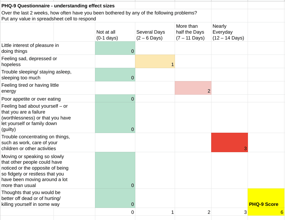
The Patient Health Questionnaire (PHQ-9) is a 9 item questionnaire that measures depression. The respondent answers each question, marks 0, 1, 2, or 3 points for each response which falls under the "not at all", "several days", "more than half the days", or "nearly everyday" categories, respectively, and then adds them up to get a total score. The score can fall between 0 and 27. Any score larger than 5, 10, 15, and 20 points is considered mild, moderate, moderately-severe, and severe depression, respectively, while scores below 5 are considered "in remission".
Given two PHQ-9 scores representing two different time points, and a mean and standard deviation, it's possible to conceptualise any change in score in terms of standard deviations of improvement. In this table, we pull data from Kroenke (2001) about the mean and standard deviation of PHQ-9 scores for patients with major depressive disorder, in order to determine that a patient whose PHQ-9 score drops from 13 to 8 has experienced 0.82 standard deviations of improvement.
| Kroenke (2001) | Major Depressive Disorder Patients |
| Mean | 17.1 |
Std Dev
| 6.1 |
| Sample Size | 41 |
| PHQ-9 score at time 1 | Z score relative to Major Depressive Disorder Patients |
13 | -0.6721311475 |
| PHQ-9 score at time 2 | |
8 | -1.491803279 |
| SD of improvement | 0.8196721311 |
In aggregate over many patients, this number becomes the effect size, reported as a standardised mean difference.
Because standardised mean differences are the way that academics report depression interventions, it's convenient to centre analysis on the impact of depression interventions for a given individual around them. Plugging these effect sizes into the equations which calculate cumulative SD-years, as described above, answers the question of "how many standard deviations of improvement does the depression intervention achieve over time".
This is the end of the section which sets out introductory tools and background material. Next we will consider one of the issues with using effect sizes, which impacts the SD-years framework. Finally, we will set out some tools which help with converting between this framework and other approaches.
5 Issues with the SD-years framework: Floor and Ceiling effects, non-normal distributions, and inclusion criteria can distort effect size measures
A problem with a standardised mean difference approach to depression is that the construct of standardised mean differences, designed with normal distributions in mind, are best used on normal-looking distributions which are symmetric and unimodal. The distribution of scores on depression questionnaires is not normal-looking for all populations.
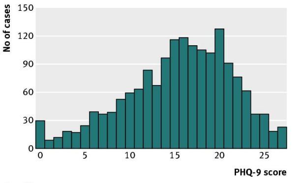
Researchers leading studies which only admit depressed patients may not find this to be a problem, because the scores of populations of people who are diagnosed with depression do fall into a classic normal distribution.
Figure: Sedgwick, P. (2012). PHQ-9 scores in patient samples that are diagnosed with depression. These data are reasonably close to normally distributed. (Note that we still have some people with depression scoring 0 on this particular questionnaire. It could be because the inclusion criteria was clinical treatment referrals and prescriptions, not the questionnaire itself, so there's no sharp cutoff. It's also possible that time passed since the diagnosis and the questionnaire, during which there may have been treatment or spontaneous remission).
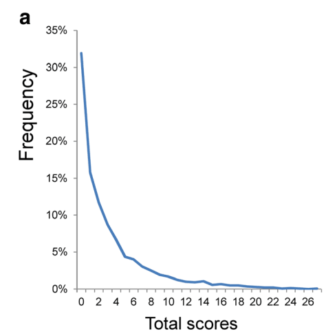
However, most people are not depressed, and depression questionnaires do not measure any states happier than "zero depression", creating a large floor effect. Let's take a look at how people in the general population tend to respond to a 9 item Patient Health Questionnaire for depression (PHQ-9).
Figure: Distributional patterns of item responses and total scores on the PHQ-9 in the general population: data from the National Health and Nutrition Examination Survey. This data is from a general population which includes both depressed and non-depressed people. As you can see, it is not normally distributed at all.
Because of how the floor effect "squishes" the data against the left size, the stronger the floor effect, the smaller the standard deviation. Because Standardised Mean Difference is calculated by dividing the difference in means by the standard deviation, an artificially low standard deviation created by a strong floor effect can inflate the effect sizes and other metrics using standardised difference from the mean.
We can observe this "squishing" by comparing the means and standard deviations in different populations. Kroenke (2001) administered the PHQ-9 alongside structured interviews with mental health professionals to 580 patients from the general population (who were in the hospital for a variety of reasons, not just depression). The following table displays the means and standard deviations for patients which the mental health professionals diagnosed with major depressive disorder, other depressive disorder, and no depressive disorder. As you can see, the non-depressed patients have a "squished" standard deviation, as do to a lesser extent the patients with "other depressive disorders", relative to the patients with major depressive disorder.
| Data from Kroenke (2001) | Major Depressive Disorder Patients | Other Depressive Disorder Patients | Non Depressed Patients | Entire population combined |
| Mean | 17.1 | 10.4 | 3.3 | 5.071206897 |
| Std Dev | 6.1 | 5.4 | 3.8 | 5.7959 |
| Sample Size | 41 | 65 | 474 | 580 |
When we use these figures to calculate the standard deviations of improvement for our hypothetical patients, we see that the degree of improvement gets inflated if we are using population norms with "squished" distributions.
| PHQ-9 score at time 1 | Z score relative to Major Depressive Disorder Patients | Z score relative to Other Depressive Disorder Patients | Z score relative to Non Depressed Patients | Z score relative to entire population (combined) | Diagnosis |
11 | -1 | 0.11 | 2.03 | 1.02 | moderate |
| PHQ-9 score at time 2 | |||||
7.95 | -1.5 | -0.45 | 1.22 | 0.50 | mild |
| SD of improvement | 0.5 | 0.56 | 0.80 | 0.53 |
This table models a hypothetical patient's raw PHQ-9 score dropping from 11 to 7.95, from "moderately" to "mildly" depressed. In patients with major depressive disorder (mean 17.1, sd 6.1), a score of 11 falls 1 standard deviation below the mean, while a score of 7.95 falls 1.5 standard deviations below the mean, which implies that the hypothetical patient improved by 0.5 standard deviations, relative to the population of patients with major depression. However, if we compare the same patient to a population of "non-depressed patients" with a narrower standard deviation of 3.8, the same patient is counted as having experienced 0.8 standard deviations of improvement. The table demonstrates how differing populations drawn from different inclusion criteria can change the headline effect size in a scientific paper.
This can pose a problem when we want to aggregate data across multiple studies. Effect sizes are the main tool we have to aggregate across scales, but because each study uses different "inclusion criteria" to identify depressed patients, it's very possible for different studies to show different ceiling or floor or other selection effects which may artificially narrow their standard deviations, which result in effect sizes which are not truly comparable. An example of this creating problems in a real-world study can be found in Appendix B. See also recent discussion between GiveWell and HLI regarding potentially distortionary floor effects on life satisfaction scales.
When comparing between scales and studies, we must therefore use extreme caution in interpreting effect sizes even in cases where a study is well designed and high powered. We are alert to the possibility of inflated effect sizes in any scenario where the mean of the sample seems too close to the edge of the scale, causing ceiling and floor effects which squish the standard deviation. This can be remedied by trying to get a sense for what scores mean in an absolute sense and what a normal standard deviation should be for a given scale before interpreting data from studies which use it. Some methods by which we can understand what the meaning of a score in an absolute sense might be will be discussed in later sections.
Next we will set out some tools which help with converting between this framework and other approaches.
6 Converting between effect sizes and the Remission, Relapse, and The "Number Needed To Treat" framework
As mentioned earlier, in the academic literature, the impact and time course of treatment is not reported in SD-years, but in terms of remission, relapse, and Number Needed to Treat (NNT).
While our opinion is that the SD-years framework is a more robust way to think about the effect of these interventions, we'd like to be able to convert between these frameworks, in order to be able to use more of the existing academic literature, and to communicate our results in a format more familiar to academics and clinicians. The following are tools to facilitate such conversion. All of these tools rely on assumptions that the sample is normally distributed.
Remission Rate
The "Remission Rate" is the proportion of patients who have improved beyond a given threshold. When a patient recovers without treatment, it's sometimes called "spontaneous remission".
The formula
Remission rate = normdist(c,𝛍,𝜎,TRUE)
uses a cumulative distribution function to calculate the remission rate of a normally distributed population, given a mean 𝛍, standard deviation 𝜎, and cutoff c. This can be used to calculate remission rates for both intervention and control groups, which can be used to calculate NNT.
Number Needed to Treat (NNT)
The "Number Needed to Treat" refers to the number of patients one would need to treat to counterfactually achieve one additional case of remission. It is calculated using the formula:
NNT = 1 / (remission rate in the treatment group - remission rate in the control group)
If you know both remission rates, you can put them into this formula. However, sometimes academic literature will only give you the remission rate of one of the two groups (usually the treatment group). In either case, it's possible to estimate the NNT.
If you have an effect size SMD, and a remission rate for a control group RMC it is possible to estimate NNT using the formula:
If you have an effect size SMD, and a remission rate for a treatment group RMT , it is possible to estimate NNT using the formula:
NNT = 1/{RMT-normsdist[SMD-normsinv(RMT)]}
These formulas are grounded in arguments by Furukawa (2011) about relating effect size and NNT, which we found compelling. We've sanity checked them against a data table produced by Furukawa (1999) and converged on the same answers.
Relapse Rate
The "Relapse Rate" refers to patients who were formerly treated, but have relapsed into depression after some time has passed.
Sometimes, academic papers will report means and standard deviations for treatment effects, but only report "relapse rate" when it comes to longitudinal follow-up. If it feels safe to make a reasonable guess about what the standard deviation 𝜎followup of the follow-up sample scores probably is, it is possible to derive the mean of the follow-up sample from the remission and relapse rates. This can be done using the formula:
𝛍followup=c-normsinv(RMT*(1-RLF))*𝜎followup
using remission cutoff c, remission rate for the treatment group before followup RMT, relapse rate at followup RLF, and the standard deviation at followup 𝜎followup.
Armed with an estimate of 𝜎followup and 𝛍followup, and given 𝜎control and 𝛍control it is possible to derive an effect size at follow-up using standard SMD calculators such as hedge's g. This can be paired with the effect size at treatment to calculate a decay rate which can fit into the SD-years framework. (Disclaimer: These equations were created by me and haven't been checked by a statistician.)
Together, these formulas make it possible to pull SMD effect sizes from papers that report results in remission and relapse rates, which allows us to incorporate data from such sources into the SD-years framework. They also allow us to convert the opposite way, from SMD effect sizes to remission rates, relapse rates, and NNT.
7 Using Z scores / standard scores to create conversion tables
In the previous sections we have described how to use standardised mean difference effect size measures, as well as some of the dangers in taking them at face value. One way we might avoid falling prey to statistical artefacts is to have large universal conversion tables which help us anchor different scales to each other. In other words, rather than relying on relative measures which give different answers depending on the population standard deviation, we could attempt to have a single "absolute" scale which could be converted into a variety of relative scales.
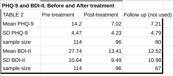
In Titov (2011), a single group of patients took both the Patient Health Questionnaire-9 Item (PHQ-9) and Beck Depression Inventory– II (BDI-II) before and after receiving treatment in an 8 week program, as well as again during a post-treatment follow-up six or eight months later. (The post-treatment follow data seems to mix patients which were followed up with six months later and patients which were followed up with eight months later in the same sample).
Because the same patients took two different questionnaires, we can know that the distribution of scores for both tests reflect a population in identical states of depression. This creates an opportunity to create a conversion scale between the BDI-II and the PHQ-9, allowing us to compare between papers which use these two different questionnaires without interference from potentially distorting effects from differences in their respective populations. This method can be useful as a sanity check against effect sizes when reading papers.
We have created a conversion table between the BDI-II and the PHQ-9. Means and standard deviations were used to assign each data point a Z score, which represents their distance in standard deviations from the mean. A given raw score x can be converted to a z score using the equation:
Z score = (x-𝛍)/𝜎
where 𝛍 and 𝜎 are the mean and standard deviation of the sample, respectively.
Points on the scale with a similar Z score are equivalent to each other. Colours represent the "severity cutoffs" arbitrarily chosen by the creators of the scale.
For the BDI-II: Red: severe; Orange: moderate; Yellow: mild; Green: minimal.
For the PHQ-9: Red: severe; Pink: moderately-severe; Orange: moderate; Yellow: mild; Green: minimal.
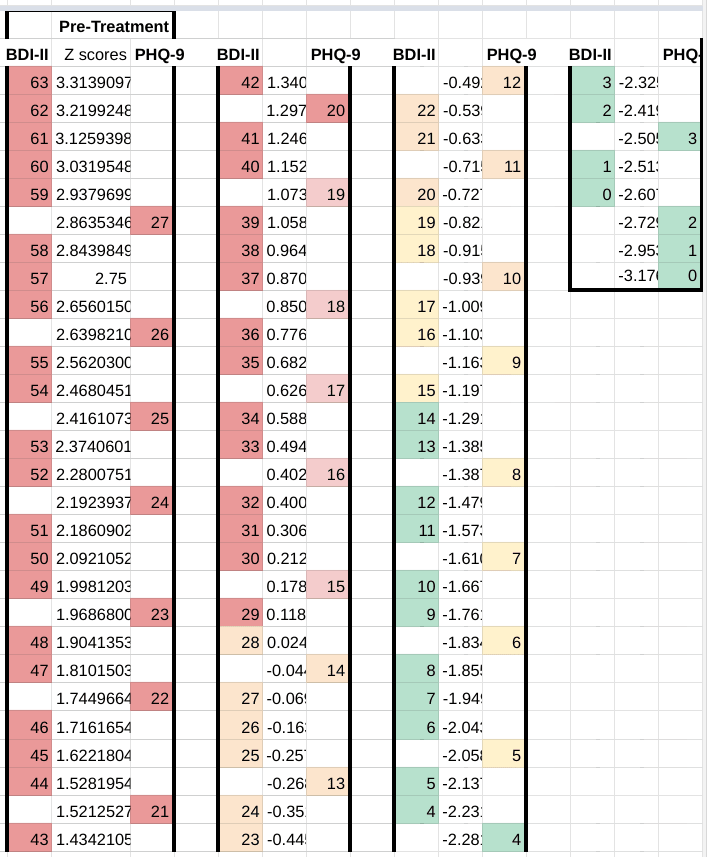
Using this chart, we can see that a PHQ-9 score of 27 corresponds to a BDH-II score of between 58 and 59, and vice versa.
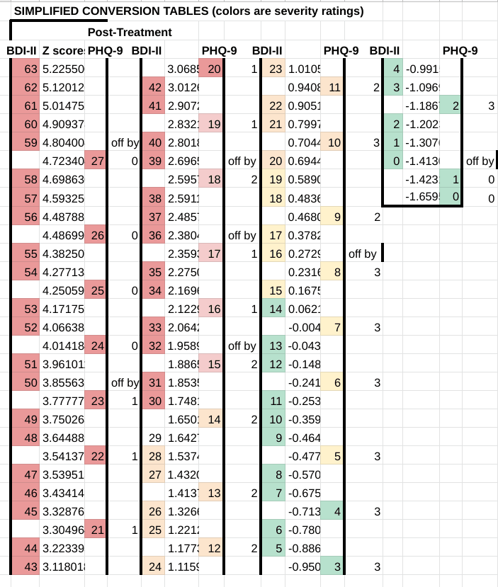
We can use a similar methodology on the post-treatment data to make a second chart, as a robustness check. It looks pretty good - PHQ-9 to BDI-II conversions are never off from pretreatment by more than 3 points, which is only 0.28 sd and it mostly only happens at the "non-depressed" end of the scale, where you'd expect assumptions of normality to stop working anyway because of the treated group hitting floor effects.
Here's some reasons why we might not trust this scale: The abstract says that the BDI-II categorizes more cases as severe than the PHQ-9, but the inclusion criteria excludes people experiencing severe depression and suicidal ideation (defined as a total PHQ-9 score > 22 or answering "more than half the days" on Question 9 which asks explicitly about suicidal ideation) from the study. The BDI-II also has a questions about suicide, but in the PHQ-9 this is one of the 9 equally weighted questions whereas in the BDI-II this is one of the 21 equally weighted questions, so excluding suicidal patients might lower severe-as-per-PHQ-9 cases disproportionately. It's also a little unclear if they actually used PHQ-9 specifically and not BDI-II for exclusion criteria. Would excluding suicidal patients (who I suspect would score proportionately higher on the PHQ-9 than the BDI-II) meaningfully distort the results? It's hard to say.
General purpose tool for converting between scales
In the hopes that future researchers will be able to use more absolute measures to provide sanity checks against effect sizes, we've built a general purpose tool to facilitate making conversion between scales. If you specify the mean and standard deviation of any two scales, and provide the range of possible scores, the tool will automatically generate a conversion table. This will not work if the underlying data does not roughly follow a normal distribution. It also will not work if the measuring instruments in question are not actually measuring roughly the same stable, tightly correlated underlying thing in roughly similar populations. (Some keywords for finding statistical tools to figure out the latter include "construct validity", "test-retest reliability", and "internal consistency"). The tool which we developed has not seen much use, and, if not for time constraints, we would subject it to further validations.
Closing Thoughts
In the coming months, we hope to finalise our cost-effective analysis on StrongMinds. The work will make use of these methodological tools. In explaining the tools we use, we hope to empower other researchers to understand our work and check it for errors, as well as to build upon these methodologies - whether within mental health, or within other cause areas which may share similar analytical challenges.
Acknowledgements
This post was authored by Ishaan Guptasarma, with thanks to the following for their comments and input:
- other members of the SoGive community
- our contacts at HLI
Citations
Spreadsheet which accompanies this document
Impact Analysis Toolkit - Accompanying Spreadsheet
Citations to EA sources
McGuire, J. (2021). Cost Effectiveness Analysis: StrongMinds. Happier Lives Institute
Response to GiveWell's assessment of StrongMinds - Happier Lives Institute
Academic citations
Sedgwick, P. (2012). The normal distribution. BMJ, 345.
Furukawa, T. A. (1999). From effect size into number needed to treat. The Lancet, 353(9165), 1680.
Metapsy database citations
Pim Cuijpers , Clara Miguel , Marketa Ciharova , David Ebert , Mathias Harrer , Eirini Karyotaki (2022) . Database of transdiagnostic psychotherapy trials for depression and anxiety. Part of the Metapsy project (Version 22.0.5 ). URL docs.metapsy.org/databases/depression-anxiety-transdiagnostic. DOI https://doi.org/10.5281/zenodo.7243836 .
Pim Cuijpers , Clara Miguel , Mathias Harrer , Constantin Yves Plessen , Marketa Ciharova , David Ebert , Eirini Karyotaki (2022) . Database of depression psychotherapy trials with control conditions. Part of the Metapsy project (Version 22.0.2 ). URL docs.metapsy.org/databases/depression-psyctr. DOI https://doi.org/10.5281/zenodo.7254845 .
Pim Cuijpers , Clara Miguel , Eirini Karyotaki (2022) . Database of depression psychotherapy trials in inpatient settings. Part of the Metapsy project (Version 22.2.1 ). URL docs.metapsy.org/databases/depression-inpatients. DOI https://doi.org/10.5281/zenodo.6881064 .
Harrer, M., Sprenger, A. A. Kuper, P., Karyotaki, E., Cuijpers, P. (2022). metapsyData: Access the Meta-Analytic Psychotherapy Databases in R. URL data.metapsy.org.
Other
Beck Depression Inventory– II (BDI-II)
Appendix A: Decay equations
The decay of effect size over time is modelled using the decay equation
d(t)=d(0)*bt
Where d(0) is the effect size immediately after the intervention, and d(t) is the value when time t elapses. The value b refers to the "decay factor". This value must be a positive number less than 1, or the equation won't "decay". If b is 1, then the effect of the intervention is constant and unchanging over time, and if b > 1 then the effect will exponentially grow.
Whenever we come across a study which has measured effect size at two or more time points, we can use it to derive the constants b and d(0), and use it to model the change in the effect size from the start of the intervention to any arbitrary time period.
The rate of decay b is found using
Where dx is the effect size at time tx years after the intervention has elapsed, and dy is the effect size at time ty years after the intervention has elapsed.
The effect size at the start of the intervention d(0) is found using the equations
or
The equations should give the same answer, and this step is redundant if tx or ty are zero because they were taken immediately after the intervention).
Note: This is not what McGuire (2021 a, b) are doing to calculate decay, since they're using effect sizes from studies rather than individual time points. Instead, they're running a meta-regression between time and ln(effect size).
Appendix B: Example of ceiling effects inflating effect sizes
To illustrate the distorting effect of squished standard deviations more deeply, let's look at some examples of obvious outliers and watch this in action.
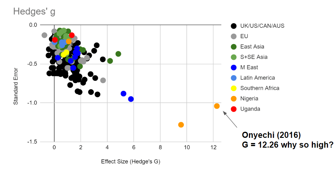
This graph displays the effect size of various therapy interventions on depression, extracted from a dataset at Metapsy (Harrer 2022, Cuijpers 2022a, Cuijpers 2022b, Cuijpers 2022c). Let's pick one of the biggest outliers (Onyechi, 2016) to get a sense of how inclusion criteria can dramatically change the standard deviation, which in turn can dramatically change the effect size. Onyechi (2016) reported post-treatment mean (s.d.) scores of 16.88 (1.56) and control mean (s.d.) scores 59.1 (3.36) for Hedges' g = 16.1. on Beck's Depression Inventory -II, a questionnaire where the maximum score is 63. (It's unclear to us why the 16.1 figure from the original study does not match with the 12.26 figure in Metapsy. Subsequent articles will discuss the difficulties of using summary statistics from meta-analyses.)
Sixteen standard deviations is impossible with a normal distribution (in a world population of 8 billion, only 15 people would fall above or below 6 standard deviations on either end of the mean on a normal distribution). Part of why we are getting an impossible number is that any standard deviations under 4 are implausibly narrow for a 63 item self report scale. Substituting in a more realistic standard deviation of 10 would give Hedges g = 4.22 (which is still very implausible but less impossible). It's unclear why Onyechi, 2016 got such low standard deviations - one possible explanation might be that their patient population was so depressed that they were hitting ceiling effects (although this does not explain why the low spread persists after treatment, nor the unusually high score change - most likely multiple factors contributed to the extreme outlier).

